00045-DGL-KE 学习笔记-windows10

前言

Knowledge graphs (KGs) are data structures that store information about different entities (nodes) and their relations (edges). A common approach of using KGs in various machine learning tasks is to compute knowledge graph embeddings. DGL-KE is a high performance, easy-to-use, and scalable package for learning large-scale knowledge graph embeddings. The package is implemented on the top of Deep Graph Library (DGL) and developers can run DGL-KE on CPU machine, GPU machine, as well as clusters with a set of popular models, including TransE, TransR, RESCAL, DistMult, ComplEx, and RotatE.

DGL-KE 代码仓库链接: https://github.com/awslabs/dgl-ke .

操作系统：Windows 10 家庭版

参考文档

项目仓库

Documentation

DGL-ke architecture
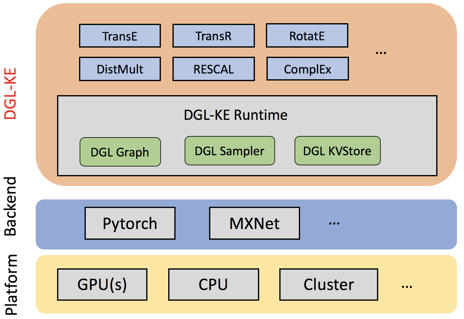
Figure: DGL-KE Overall Architecture

Currently DGL-KE support three tasks:

Training, trains KG embeddings using dglke_train(single machine) or dglke_dist_train(distributed environment).
Evaluation, reads the pre-trained embeddings and evaluates the embeddings with a link prediction task on the test set using dglke_eval.
Inference, reads the pre-trained embeddings and do the entities/relations linkage predicting inference tasks using dglke_predict or do the embedding similarity inference tasks using dglke_emb_sim.

A Quick Start

To install the latest version of DGL-KE run:

1 2	sudo pip3 install dgl sudo pip3 install dglke

Train a transE model on FB15k dataset by running the following command:

1
2
3

DGLBACKEND=pytorch dglke_train --model_name TransE_l2 --dataset FB15k --batch_size 1000 \
--neg_sample_size 200 --hidden_dim 400 --gamma 19.9 --lr 0.25 --max_step 500 --log_interval 100 \
--batch_size_eval 16 -adv --regularization_coef 1.00E-09 --test --num_thread 1 --num_proc 8

This command will download the FB15k dataset, train the transE model and save the trained embeddings into the file.

Performance and Scalability

DGL-KE is designed for learning at scale. It introduces various novel optimizations that accelerate training on knowledge graphs with millions of nodes and billions of edges. Our benchmark on knowledge graphs consisting of over 86M nodes and 338M edges shows that DGL-KE can compute embeddings in 100 minutes on an EC2 instance with 8 GPUs and 30 minutes on an EC2 cluster with 4 machines (48 cores/machine). These results represent a 2×∼5× speedup over the best competing approaches.

vs-gv-fb15k
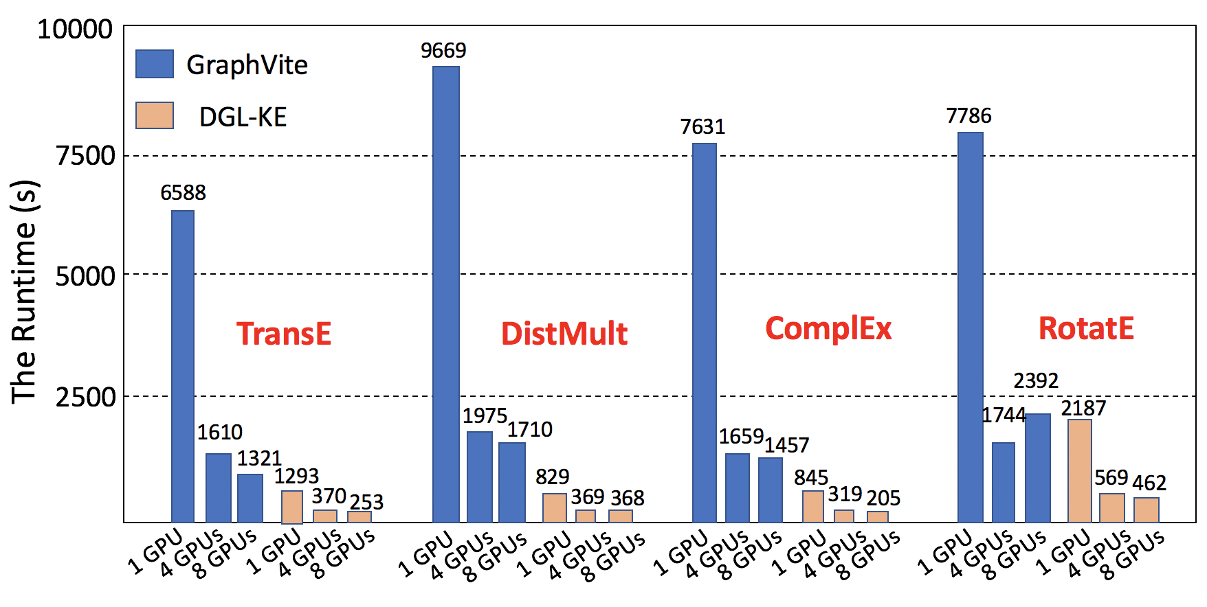
Figure: DGL-KE vs GraphVite on FB15k

vs-pbg-fb
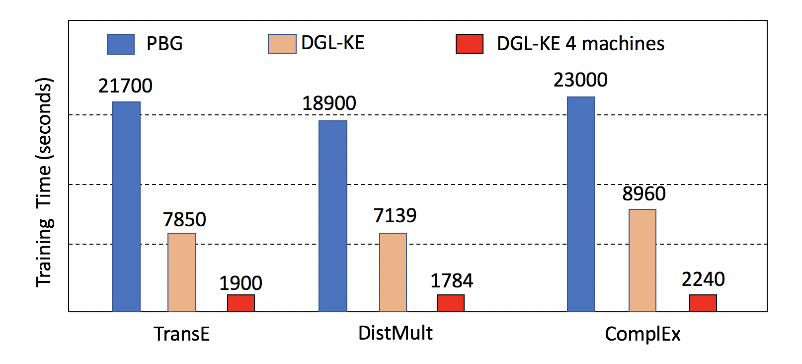
Figure: DGL-KE vs Pytorch-BigGraph on Freebase

Learn more details with our documentation! If you are interested in the optimizations in DGL-KE, please check out our paper for more details.

Cite

If you use DGL-KE in a scientific publication, we would appreciate citations to the following paper:

@inproceedings{DGL-KE,
author = {Zheng, Da and Song, Xiang and Ma, Chao and Tan, Zeyuan and Ye, Zihao and Dong, Jin and Xiong, Hao and Zhang, Zheng and Karypis, George},
title = {DGL-KE: Training Knowledge Graph Embeddings at Scale},
year = {2020},
publisher = {Association for Computing Machinery},
address = {New York, NY, USA},
booktitle = {Proceedings of the 43rd International ACM SIGIR Conference on Research and Development in Information Retrieval},
pages = {739–748},
numpages = {10},
series = {SIGIR '20}
}

License

This project is licensed under the Apache-2.0 License.

DGL-KE Documentation

原文档地址: https://dglke.dgl.ai/doc/ .

Knowledge graphs (KGs) are data structures that store information about different entities (nodes) and their relations (edges). A common approach of using KGs in various machine learning tasks is to compute knowledge graph embeddings. DGL-KE is a high performance, easy-to-use, and scalable package for learning large-scale knowledge graph embeddings. The package is implemented on the top of Deep Graph Library (DGL) and developers can run DGL-KE on CPU machine, GPU machine, as well as clusters with a set of popular models, including TransE, TransR, RESCAL, DistMult, ComplEx, and RotatE.

Performance and Scalability

DGL-KE is designed for learning at scale. It introduces various novel optimizations that accelerate training on knowledge graphs with millions of nodes and billions of edges. Our benchmark on knowledge graphs consisting of over 86M nodes and 338M edges shows that DGL-KE can compute embeddings in 100 minutes on an EC2 instance with 8 GPUs and 30 minutes on an EC2 cluster with 4 machines (48 cores/machine). These results represent a 2×∼5× speedup over the best competing approaches.

DGL-KE vs Graphvite

DGL-KE vs Pytorch-Biggraph

Get started with DGL-KE!

Installation Guide

原文档地址: https://dglke.dgl.ai/doc/install.html .

This topic explains how to install DGL-KE. We recommend installing DGL-KE by using pip and from the source.

System requirements

DGL-KE works with the following operating systems:

Ubuntu 16.04 or higher version
macOS x

DGL-KE requires Python version 3.5 or later. Python 3.4 or earlier is not tested. Python 2 support is coming.

DGL-KE supports multiple tensor libraries as backends, e.g., PyTorch and MXNet. For requirements on backends and how to select one, see Working with different backends. As a demo, we install Pytorch using pip:

1	sudo pip3 install torch

Install DGL

DGL-KE is implemented on the top of DGL (0.4.3 version). You can install DGL using pip:

1	sudo pip3 install dgl==0.4.3

Install DGL-KE

After installing DGL, you can install DGL-KE. The fastest way to install DGL-KE is by using pip:

1	sudo pip3 install dglke

or you can install DGL-KE from source:

1
2
3

git clone https://github.com/awslabs/dgl-ke.git
cd dgl-ke/python
sudo python3 setup.py install

Have a Quick Test

Once you install DGL-KE successfully, you can test it by the following command:

# create a new workspace
mkdir my_task && cd my_task
# Train transE model on FB15k dataset
DGLBACKEND=pytorch dglke_train --model_name TransE_l2 --dataset FB15k --batch_size 1000 \
--neg_sample_size 200 --hidden_dim 400 --gamma 19.9 --lr 0.25 --max_step 500 --log_interval 100 \
--batch_size_eval 16 -adv --regularization_coef 1.00E-09 --test --num_thread 1 --num_proc 8

This command will download the FB15k dataset, train the transE model on that, and save the trained embeddings into the file. You could see the following output at the end:

-------------- Test result --------------
Test average MRR : 0.47221913961451095
Test average MR : 58.68289854581774
Test average HITS@1 : 0.2784276548560207
Test average HITS@3 : 0.6244265375564998
Test average HITS@10 : 0.7726295474936941
-----------------------------------------

Introduction to Knowledge Graph Embedding

原文档地址: https://dglke.dgl.ai/doc/kg.html .

Knowledge Graphs (KGs) have emerged as an effective way to integrate disparate data sources and model underlying relationships for applications such as search. At Amazon, we use KGs to represent the hierarchical relationships among products; the relationships between creators and content on Amazon Music and Prime Video; and information for Alexa’s question-answering service. Information extracted from KGs in the form of embeddings is used to improve search, recommend products, and infer missing information.

What is a graph

A graph is a structure used to represent things and their relations. It is made of two sets - the set of nodes (also called vertices) and the set of edges (also called arcs). Each edge itself connects a pair of nodes indicating that there is a relation between them. This relation can either be undirected, e.g., capturing symmetric relations between nodes, or directed, capturing asymmetric relations. For example, if a graph is used to model the friendship relations of people in a social network, then the edges will be undirected as they are used to indicate that two people are friends; however, if the graph is used to model how people follow each other on Twitter, the edges will be directed. Depending on the edges’ directionality, a graph can be directed or undirected.

Graphs can be either homogeneous or heterogeneous. In a homogeneous graph, all the nodes represent instances of the same type and all the edges represent relations of the same type. For instance, a social network is a graph consisting of people and their connections, all representing the same entity type. In contrast, in a heterogeneous graph, the nodes and edges can be of different types. For instance, the graph for encoding the information in a marketplace will have buyer, seller, and product nodes that are connected via wants-to-buy, has-bought, is-customer-of, and is-selling edges.

Finally, another class of graphs that is especially important for knowledge graphs are multigraphs. These are graphs that can have multiple (directed) edges between the same pair of nodes and can also contain loops. These multiple edges are typically of different types and as such most multigraphs are heterogeneous. Note that graphs that do not allow these multiple edges and self-loops are called simple graphs.

What is a Knowledge Graph

In the earlier marketplace graph example, the labels assigned to the different node types (buyer, seller, product) and the different relation types (wants-to-buy, has-bought, is-customer-of, is-selling) convey precise information (often called semantics) about what the nodes and relations represent for that particular domain. Once this graph is populated, it will encode the knowledge that we have about that marketplace as it relates to types of nodes and relations included. Such a graph is an example of a knowledge graph.

A knowledge graph (KG) is a directed heterogeneous multigraph whose node and relation types have domain-specific semantics. KGs allow us to encode the knowledge into a form that is human interpretable and amenable to automated analysis and inference. KGs are becoming a popular approach to represent diverse types of information in the form of different types of entities connected via different types of relations.

When working with KGs, we adopt a different terminology than the traditional vertices and edges used in graphs. The vertices of the knowledge graph are often called entities and the directed edges are often called triplets and are represented as a (h, r, t) tuple, where h is the head entity, t is the tail entity, and r is the relation associating the head with the tail entities. Note that the term relation here refers to the type of the relation (e.g., one of wants-to-buy, has-bought, is-customer-of, and is-selling).

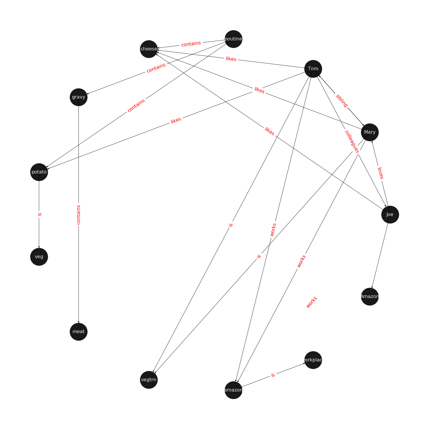
Let us examine a directed multigraph in an example, which includes a cast of characters and the world in which they live.

Scenario:

Mary and Tom are siblings and they both are are vegetarians, who like potatoes and cheese. Mary and Tom both work at Amazon. Joe is a bloke who is a colleague of Tom. To make the matter complicated, Joe loves Mary, but we do not know if the feeling is reciprocated.

Joe is from Quebec and is proud of his native dish of Poutine, which is composed of potato, cheese, and gravy. We also know that gravy contains meat in some form.

Joe is excited to invite Tom for dinner and has sneakily included his sibling, Mary, in the invitation. His plans are doomed from get go as he is planning to serve the vegetarian siblings his favourite Quebecois dish, Poutine.

Oh! by the way, a piece of geography trivia: Quebec is located in a province of the same name which in turn is located in Canada.

There are several relationships in this scenario that are not explicitly mentioned but we can simply infer from what we are given:

Mary is a colleague of Tom.
Tom is a colleague of Mary.
Mary is Tom’s sister.
Tom is Mary’s brother.
Poutine has meat.
Poutine is not a vegetarian dish.
Mary and Tom would not eat Poutine.
Poutine is a Canadian dish.
Joe is Canadian.
Amazon is a workplace for Mary, Tom, and Joe.

There are also some interesting negative conclusions that seem intuitive to us, but not to the machine:

Potato does not like Mary.
Canada is not from Joe.
Canada is not located in Quebec.

What we have examined is a knowledge graph, a set of nodes with different types of relations:

1-to-1: Mary is a sibling of Tom.
1-to-N: Amazon is a workplace for Mary, Tom, and Joe.
N-to-1: Joe, Tom, and Mary work at Amazon.
N-to-N: Joe, Mary, and Tom are colleagues.

There are other categorization perspectives on the relationships as well:

Symmetric: Joe is a colleague of Tom entails Tom is also a colleague of Joe.
Antisymmetric: Quebec is located in Canada entails that Canada cannot be located in Quebec.

Figure 1 visualizes a knowledge-base that describes World of Mary. For more information on how to use the examples, please refer to the code that draws the examples.

What is the task of Knowledge Graph Embedding?

Knowledge graph embedding is the task of completing the knowledge graphs by probabilistically inferring the missing arcs from the existing graph structure. KGE differs from ordinary relation inference as the information in a knowledge graph is multi-relational and more complex to model and computationally expensive. For this rest of this blog, we examine fundamentals of KGE.

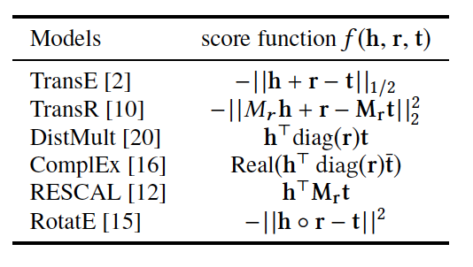
Score Function

There are different flavours of KGE that have been developed over the course of the past few years. What most of them have in common is a score function. The score function measures how distant two nodes relative to its relation type. As we are setting the stage to introduce the reader to DGL-KE, an open source knowledge graph embedding library, we limit the scope only to those methods that are implemented by DGL-KE and are listed in Figure 2.

Figure2: A list of score functions for KE papers implemented by DGL-KE

A short explanation of the score functions

Knowledge graphs that are beyond toy examples are always large, high dimensional, and sparse. High dimensionality and sparsity result from the amount of information that the KG holds that can be represented with 1-hot or n-hot vectors. The fact that most of the items have no relationship with one another is another major contributor to sparsity of KG representations. We, therefore, desire to project the sparse and high dimensional graph representation vector space into a lower dimensional dense space. This is similar to the process used to generate word embeddings and reduce dimensions in recommender systems based on matrix factorization models. I will provide a detailed account of all the methods in a different post, but here I will shortly explain how projections differ in each paper, what the score functions do, and what consequences the choices have for relationship inference and computational complexity.

TransE

TransE is a representative translational distance model that represents entities and relations as vectors in the same semantic space of dimension $\mathbb{R}^d$ , where $d$ is the dimension of the target space with reduced dimension. A fact in the source space is represented as a triplet $(h,r,t)$ where $h$ is short for head, $r$ is for relation, and $t$ is for tail. The relationship is interpreted as a translation vector so that the embedded entities are connected by relation $r$ have a short distance. In terms of vector computation it could mean adding a head to a relation should approximate to the relation’s tail, or $h+r \approx t$ . For example if $h_1=emb("Ottawa"),\ h_2=emb("Berlin"), t_1=emb("Canada"), t_2=("Germany")$ , and finally $r="CapilatOf"$ , then $h_1 + r$ and $h_2+r$ should approximate $t_1$ and $t_2$ respectively. TransE performs linear transformation and the scoring function is negative distance between $h+r$ and $t$ , or $f=-\|h+r-t\|_{\frac{1}{2}}$

Figure 3: TransE

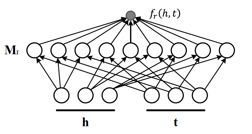
TransR

TransE cannot cover a relationship that is not 1-to-1 as it learns only one aspect of similarity. TransR addresses this issue with separating relationship space from entity space where $h, t \in \mathbb{R}^k$ and $r \in \mathbb{R}^d$ . The semantic spaces do not need to be of the same dimension. In the multi-relationship modeling we learn a projection matrix $M\in \mathbb{R}^{k \times d}$ for each relationship that can project an entity to different relationship semantic spaces. Each of these spaces capture a different aspect of an entity that is related to a distinct relationship. In this case a head node $h$ and a tail node $t$ in relation to relationship $r$ is projected into the relationship space using the learned projection matrix $M_r$ as $h_r=hM_r$ and $t_r=tM_r$ respectively. Figure 5 illustrates this projection.

Let us explore this using an example. Mary and Tom are siblings and colleagues. They both are vegetarians. Joe also works for Amazon and is a colleague of Mary and Tom. TransE might end up learning very similar embeddings for Mary, Tom, and Joe because they are colleagues but cannot recognize the (not) sibling relationship. Using TransR, we learn projection matrices: $M_{sib},\ M_{clg}$ and $M_{vgt}$ that perform better at learning relationship like (not)sibling.

The score function in TransR is similar to the one used in TransE and measures euclidean distance between $h+r$ and $t$ , but the distance measure is per relationship space. More formally: $f_r=\|h_r+r-t_r\|_2^2$

Figure 4: TransR projecting different aspects of an entity to a relationship space.

Another advantage of TransR over TransE is its ability to extract compositional rules. Ability to extract rules has two major benefits. It offers richer information and has a smaller memory space as we can infer some rules from others.

Drawbacks

The benefits from more expressive projections in TransR adds to the complexity of the model and a higher rate of data transfer, which has adversely affected distributed training. TransE requires $O(d)$ parameters per relation, where $d$ is the dimension of semantic space in TransE and includes both entities and relationships. As TransR projects entities to a relationship space of dimension $k$ , it will require $O(kd)$ parameters per relation. Depending on the size of k, this could potentially increase the number of parameters drastically. In exploring DGL-KE, we will examine benefits of DGL-KE in making computation of knowledge embedding significantly more efficient.

TransE and its variants such as TransR are generally called translational distance models as they translate the entities, relationships and measure distance in the target semantic spaces. A second category of KE models is called semantic matching that includes models such as RESCAL, DistMult, and ComplEx.These models make use of a similarity-based scoring function.

The first of semantic matching models we explore is RESCAL.

RESCAL

RESCAL is a bilinear model that captures latent semantics of a knowledge graph through associate entities with vectors and represents each relation as a matrix that models pairwise interaction between entities.

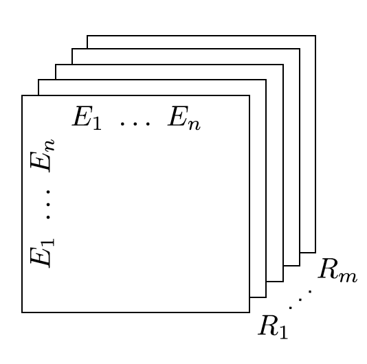
Multiple relations of any order can be represented as tensors. In fact $n-dimensional$ tensors are by definition representations of multi-dimensional vector spaces. RESCAL, therefore, proposes to capture entities and relationships as multidimensional tensors as illustrated in figure 5.

RESCAL uses semantic web’s RDF formation where relationships are modeled as $(subject, predicate, object)$ . Tensor $\mathcal{X}$ contains such relationships as $\mathcal{X}_{ijk}$ between $i$ th and $j$ th entities through $k$ th relation. Value of $\mathcal{X}_{ijk}$ is determined as:

$\begin{split}\mathcal{X}_{ijk} = \begin{cases} 1\ &\quad\text{if }(e_i, r_k, e_j)\text{ holds}\\ 0\ &\quad\text{if }(e_i, r_k, e_j)\text{ does not hold} \end{cases}\end{split}$

Figure 5: RESCAL captures entities and their relations as multi-dimensional tensor

As entity relationship tensors tend to be sparse, the authors of RESCAL, propose a dyadic decomposition to capture the inherent structure of the relations in the form of a latent vector representation of the entities and an asymmetric square matrix that captures the relationships. More formally each slice of $\mathcal{X}_k$ is decomposed as a rank $-r$ factorization:

$\mathcal{X}_k \approx AR_k\mathbf{A}^\top, \text{ for } k=1, \dots, m$

where A is an $n\times r$ matrix of latent-component representation of entities and asymmetrical $r\times r$ square matrix $R_k$ that models interaction for $k_th$ predicate component in $\mathcal{X}$ . To make sense of it all, let’s take a look at an example:

$\begin{gather} Entities=\{\text{Mary :}0, \text{Tom :}1, \text{Joe :}2\} \\ Relationships=\{\text{sibling, colleague}\} \\ Relation_{k=0}^{sibling}: \text{Mary and Tom are siblings but Joe is not their sibling.} \\ Relations_{k=1}^{colleague}: \text{Mary,Tom, and Joe are colleagues}\\ \text{relationship matrices will model: }\mathcal{X_k}= \begin{bmatrix} Mary & Tom & Joe \\ Tom & Joe & Mary \\ Joe & Mary & Tom \end{bmatrix}\\ {\mathcal{X}}_{0:sibling}= \begin{bmatrix} 0 & 1 & 0\\ 0 & 0 & 1\\ 0 & 0 & 0 \end{bmatrix}\\ \mathcal{X}_{1:colleague}= \begin{bmatrix} 0 & 1 & 1\\ 1 & 0 & 1\\ 1 & 1 & 0 \end{bmatrix} \end{gather}$

Note that even in such a small knowledge graph where two of the three entities have even a symmetrical relationship, matrices $\mathcal{X}_k$ are sparse and asymmetrical. Obviously colleague relationship in this example is not representative of a real world problem. Even though such relationships can be created, they contain no information as probability of occurring is high. For instance if we are creating a knowledge graph for registered members of a website is a specific country, we do not model relations like “is countryman of” as it contains little information and has very low entropy.

Next step in RESCAL is decomposing matrices $\mathcal{X}_k$ using a rank_k decomposition as illustrated in figure 6.

Figure 6: Each of the $k$ slices of martix $\mathcal{X}$ is factorized to its k-rank components in form of a $n\times r$ entity-latent component and an asymmetric $r\times r$ that specifies interactions of entity-latent components per relation.

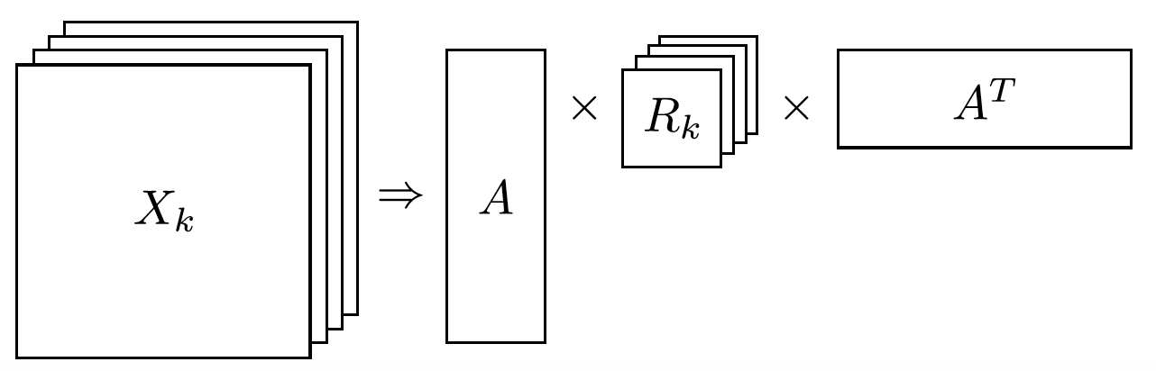
$A$ and $R_k$ are computed through solving an optimization problem that is correlated to minimizing the distance between $\mathcal{X}_k$ and $AR_k\mathbf{A}^\top$ .

Now that the structural decomposition of entities and their relationships are modeled, we need to create a score function that can predict existence of relationship for those entities we lack their mutual connection information.

The score function $f_r(h,t)$ for $h,t\in \mathbb{R}^d$ , where $h$ and $t$ are representations of head and tail entities, captures pairwise interactions between entities in $h$ and $t$ through relationship matrix $M_r$ that is the collection of all individual $R_k$ matrices and is of dimension $d\times d$ .

$f_r(h, t) = \mathbf{h}^\top M_rt = \sum_{i=0}^{d-1}\sum_{j=0}^{d-1}[M_r]_{ij}.[h]_i.[t]_j$

Figure 7 illustrates computation of the the score for RESCAL method.

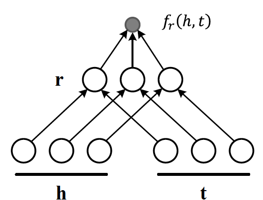
Figure 7: RESCAL

Score function $f$ requires $O(d^2)$ parameters per relation.

DistMult

If we want to speed up the computation of RESCAL and limit the relationships only to symmetric relations, then we can take advantage of the proposal put forth by DistMult, which simplifies RESCAL by restricting $M_r$ from a general asymmetric $r\times r$ matrix to a diagonal square matrix, thus reducing the number of parameters per relation to $O(d)$ . DistMulti introduces vector embedding $r \in \mathcal{R}^d$ , the score function for DistMult where $M_r=diag(r)$ is computed as:

$f_r(h,t) = \mathbf{h}^\top diag(r) t = \sum_{i=0}^{d-1}[r]_i.[h]_i.[t]_i$

Figure 8 illustrates how DistMulti computes the score by capturing the pairwise interaction only along the same dimensions of components of h and t.

Figure 8: DistMulti

A basic refresher on linear algebra

$\begin{split}if\ A=[a_{ij}]_{m\times n}= \begin{bmatrix} a_{11} & a_{12} & \dots & a_{1n} \\ a_{21} & a_{22} & \dots & a_{2n} \\ \vdots & \vdots & \ddots & \dots \\ a_{m1} & a_{m2} & \dots & a_{mn} \\ \end{bmatrix}_{m\times n} \text{ and } B=[b_{ij}]_{n\times k}= \begin{bmatrix} b_{11} & b_{12} & \dots & b_{1k} \\ b_{21} & b_{22} & \dots & b_{2k} \\ \vdots & \vdots & \ddots & \dots \\ b_{n1} & b_{n2} & \dots & b_{nk} \\ \end{bmatrix}_{n\times k}\ \\ then\ C=[c_{mk}]_{m\times k}\ such\ that\ c_{mk}=\sum_{p=1}^{k}a_{mp}b_{pk}\, thus: \\ C_{m\times k} = \begin{bmatrix} a_{11}b_{11} + \dots + a_{1n}b_{n1} & a_{11}b_{12} + \dots + a_{1n}b_{n2} & \dots & a_{11}b_{1k} + \dots + a_{1n}b_{nk} \\ a_{21}b_{11} + \dots + a_{2n}b_{n1} & a_{21}b_{12} + \dots + a_{2n}b_{n2} & \dots & a_{21}b_{1k} + \dots + a_{2n}b_{nk} \\ \vdots & \vdots & \ddots & \dots \\ a_{m1}b_{11} + \dots + a_{mn}b_{n1} & a_{m1}b_{12} + \dots + a_{mn}b_{n2} & \dots & a_{m1}b_{1k} + \dots + a_{mn}b_{nk} \\ \end{bmatrix}_{n\times k}\end{split}$

We know that a diagonal matrix is a matrix in which all non diagonal elements, $(i \neq j)$ , are zero. This reduces complexity of matrix multiplication as for diagonal matrix multiplication for diagonal matrices $A_{m\times n}$ and $B_{n\times k}$ , $C=AB= [c_{mk}]_{m\times k}$ where

$\begin{split}c_{mk} = \begin{cases} 0& \text{for }m \neq k \\ a_mb_k& \text{for }m = k \end{cases}\end{split}$

This is basically multiplying to numbers $a_{ii}$ and $b_{ii}$ to get the value for the corresponding diagonal element on $C$ .

This complexity reduction is the reason that whenever possible we would like to reduce matrices to diagonal matrices.

ComplEx

In order to model a KG effectively, models need to be able to identify most common relationship patters as laid out earlier in this blog. relations can be reflexive/irreflexive, symmetric/antisymmetric, and transitive/intransitive. We have also seen two classes of semantic matching models, RESCAL and DistMulti. RESCAL is expressive but has an exponential complexity, while DistMulti has linear complexity but is limited to symmetric relations.

An ideal model needs to keep linear complexity while being able to capture antisymmetric relations. Let us go back to what is good at DistMulti. It is using a rank-decomposition based on a diagonal matrix. We know that dot product of embedding scale well and handles symmetry, reflexity, and irreflexivity effectively. Matrix factorization (MF) methods have been very successful in recommender systems. MF works based on factorizing a relation matrix to dot product of lower dimensional matrices $\mathbf{U}\mathbf{V}^\top$ where $\mathbf{U}\mathbf{V} \in \mathbb{R}^{n\times K}$ . The underlying assumption here is that the same entity would be taken to be different depending on whether it appears as a subject or an object in a relationship. For instance “Quebec” in “Quebec is located in Canada” and “Joe is from Quebec” appears as subject and object respectively. In many link prediction tasks the same entity can assume both roles as we perform graph embedding through adjacency matrix computation. Dealing with antisymmetric relationships, consequently, has resulted in an explosion of parameters and increased complexity and memory requirements.

The goal ComplEx is set to achieve is performing embedding while reducing the number of required parameters, to scale well, and to capture antisymmetric relations. One essential strategy is to compute a joint representation for the entities regardless of their role as subject or object and perform dot product on those embeddings.

Such embeddings cannot be achieved in the real vector spaces, so the ComplEx authors propose complex embedding.

But first a quick reminder about complex vectors.

Complex Vector Space 1 is the unit for real numbers, $i=\sqrt{-1}$ is the imaginary unit of complex numbers. Each complex number has two parts, a real and an imaginary part and is represented as $c = a + bi \in \mathbb{C}$ . As expected, the complex plane has a horizontal and a vertical axis. Real numbers are placed on the horizontal axis and the vertical axis represents the imaginary part of a number. This is done in much the same way as in $x$ and $y$ are represented on Cartesian plane. An n-dimensional complex vector $\mathcal{V}\in \mathbb{C}^n$ is a vector whose elements $v_i\in \mathbb{C}$ are complex numbers.

Example:

$\begin{split}V_1 = \begin{bmatrix} 2 + 3i \\ 1 + 5i \end{bmatrix} \text{ and } V_2 = \begin{bmatrix} 2 + 3i \\ 1 + 5i \\ 3 \end{bmatrix} \text{ are in } \mathbb{C}^2\text{ and }\mathbb{C}^3\text{ respectively.}\end{split}$

$\mathbb{R} \subset \mathbb{C}$ and $\mathbb{R}^n \subset \mathbb{C}^n$ . Basically a real number is a complex number whose imaginary part has a coefficient of zero.

modulus of a complex number $z$ is a complex number as is given by $z=a+bi$ , modulus $z$ is analogous to size in vector space and is given by $\mid z\mid = \sqrt{a^2 + b^2}$

Complex Conjugate The conjugate of complex number $z=a+bi$ is denoted by $\bar{z}$ and is given by $\bar{z}=a-bi$ .

Example:

$\begin{split}\bar{V}_1 = \begin{bmatrix} 2 - 3i \\ 1 - 5i \end{bmatrix} \text{ and } \bar{V}_2 = \begin{bmatrix} 2 - 3i \\ 1 - 5i \\ 3 \end{bmatrix} \text{ are in } \mathbb{C}^2\text{ and }\mathbb{C}^3\text{ respectively.}\end{split}$

Conjugate Transpose The conjugate transpose of a complex matrix $\mathcal{A}$ , is denoted as $\mathcal{A}^*$ and is given by $\mathcal{A}^* = \mathbf{\bar{\mathcal{A}}}^\top$ where elements of $\bar{\mathcal{A}}$ are complex conjugates of $\mathcal{A}.$

Example:

$V^*_1 = \begin{bmatrix} 2 - 3i & 1 - 5i \end{bmatrix} \text{ and } V^*_2 = \begin{bmatrix} 2 - 3i & 1 - 5i & 3 \end{bmatrix} \text{ are in } \mathbb{C}^2\text{ and }\mathbb{C}^3\text{ respectively.}$

Complex dot product. aka Hermitian inner product if $\mathbf{u}$ and $\mathbf{c}$ are complex vectors, then their inner product is defined as $\langle \mathbf{u}, \mathbf{v} \rangle = \mathbf{u}^*\mathbf{v}$ .

Example:

$\begin{split}u = \begin{bmatrix} 2 + 3i \\ 1 + 5i \end{bmatrix} \text{ and } v = \begin{bmatrix} 1 + i \\ 2 + 2i \end{bmatrix} \text{ are in } \mathbb{C}^2\text{ and }\mathbb{C}^3\text{ respectively.} \\ \text{ then }u^*= \begin{bmatrix} 2 - 3i & 1 - 5i \end{bmatrix} \text{ and } \\ \langle u,v \rangle = u^*v = \begin{bmatrix} 2 - 3i & 1 - 5i \end{bmatrix} \begin{bmatrix} 1 + i \\ 2 + 2i \end{bmatrix} = (2-3i)(1+i)+(1-5i)(2+2i)=[4-13i]\end{split}$

Definition: A complex matrix $A$ us unitary when $A^{-1} = A^*$

Example: $A = \frac{1}{2}\begin{bmatrix}1+i & 1-i \\1-i & 1+i\end{bmatrix}$

Theorem: An $n \times n$ complex matrix $A$ is unitary $\iff$ its rows or columns form an orthanormal set in $\mathcal{C}^n$

Definition: A square matrix $A$ is Hermitian when $A=A^*$

Example: $A = \begin{bmatrix}a_1 & b_1+b_2i \\b_1+b_2i & d+1\end{bmatrix}$

Theorem: Matrix $A$ is Hermitian $\iff$ :

$a_{ii} \in \mathbb{R}$
$a_{ij}$ is complex conjugate of $a_{ji}$

Theorem: If $A$ is a Hermirian matrix, then its eigenvalues are real numbers.

Theorem: Hermitian matrices are unitarity diagonizable.

Definitions: A squared matrix A is unitarily diagonizable when there exists a unitary matrix $P$ such that $P^{-1}AP$ .

Diagonizability can be extended to a larger class of matrices, called normal matrices.

Definition: A square complex matrix A is called normal when it commutes with its conjugate transpose. $AA^*=A^*A$ .

Theorem: A complex matrix $A$ is normal $\iff A$ is diagonizable.

This theorem plays a crucial role in ComplEx paper.

Eigen decomposition for entity embedding

The matrix decomposition methods have a long history in machine learning. Using embeddings based decomposition in the form of $X=EWE^{-1}$ for square symmetric matrices can be represented as eigen decomposition $X=Q\Lambda Q^{-1}$ where $Q$ is orthogonal $(Q^{-1} = Q^\top)$ and $\Lambda = diag(\lambda)$ and $\lambda_i$ is an eigenvector of $X$ .

As ComplEx targets to learn antisymmetric relations, and eigen decomposition for asymmetric matrices does not exist in real space, the authors extend the embedding representation to complex numbers, where they can factorize complex matrices and benefit from efficient scaling and distribution of matrix multiplication while being able to capture antisymmetric relations. This asymmetry is resulted from the fact that dot product of complex matrices involves conjugate transpose.

We are not done yet. Do you remember in RESCAL the number of parameters was $O(d^2)$ and DistMulti reduce that to a linear relation of $O(d)$ by limiting matrix $M_r$ to be diagonal?. Here even with complex eigenvectors $E \in \mathcal{C}^{n \times n}$ , inversion of $E$ in $X=EWE^{*}$ explodes the number of parameters. As a result we need to find a solutions in which W is a diagonal matrix, and $E = E^*$ , and $X$ is asymmetric, so that we

computation is minimized,
there is no need to compute inverse of $E$ , and
antisymmetric relations can be captures. We have already seen the solution in the complex vector space section. The paper does construct the decomposition in a normal space, a vector space composed of complex normal vectors.

The Score Function

A relation between two entities can be modeled as a sign function, meaning that if there is a relation between a subject and an object, then the score is 1, otherwise it is -1. More formally, $Y_{so}\in \{-1, 1\}$ . The probability of a relation between two edntities to exist is then given by sigmoid function: $P(Y_{so}=1) = \sigma(X_{so})$ .

This probability score requires $X$ to be real, while $EWE^*$ includes both real and imaginary components. We can simply project the decomposition to the real space so that $X =Re(EWE^*)$ . the score function of ComlEx, therefore is given by:

$f_r(h, t) = Re(h^\top diag(r) \bar{t}) = Re(\sum_{i=0}^{d-1}[r]_i.[h]_i.[\bar{t}]_i)$

and since there are no nested loops, the number of parameters is linear and is given by $O(d)$ .

RotateE

Let us reexamine translational distance models with the ones in latest publications on relational embedding models (RotateE). Inspired by TransE, RotateE veers into complex vector space and is motivated by Euler’s identity, defines relations as rotation from head to tail.

Euler’s Formula

$e^x$ can be computed using the infinite series below:

$e^x = 1 + \frac{x}{1!} +\frac{x^2}{2!} + \frac{x^3}{3!} + \frac{x^4}{4!}+ \frac{x^5}{5!} + \frac{x^6}{6!} + \frac{x^7}{7!} + \frac{x^8}{8!} + \dots$

replacing $x$ with $ix$ entails:

$\begin{split}e^{(ix)} = 1 + \frac{ix}{1!} - \frac{x^2}{2!} - \frac{ix^3}{3!} + \frac{x^2}{4!} + \frac{ix^5}{5!} - \frac{x^6}{6!} - \frac{ix^7}{3!} + \frac{x^8}{8!} + \dots\\\end{split}$

Computing $i$ to a sequence of powers and replacing the values in $e^{ix}$ , the results in:

$\begin{split}i^2=-1,\ i^3=i^2i=-i,\ i^4=ii^3=-1^2=1,\ i^5=i^4i=i,\ i^6=i^5i=i^2=-1,\ \dots\\ e^{(ix)} = 1 + \frac{ix}{1!} +\frac{i^2x^2}{2!} + \frac{i^3x^3}{3!} + \frac{i^4x^4}{4!} + \frac{i^5x^5}{5!} + \frac{i^6x^6}{6!} + \dots\\\end{split}$

rearranging the series and factoring $i$ in terms that include it:

$\begin{split}1 - \frac{x^2}{2!} + \frac{x^4}{4!} - \frac{x^6}{6!} + \frac{x^8}{8!} +i\left(\frac{x}{1!} - \frac{x^3}{3!} + \frac{x^5}{5!} - \frac{x^7}{7!} \right)\text{ (1)}\\\end{split}$

$sin$ and $cosin$ representation as series are given by:

$\begin{split}sin(x) = \frac{x}{1!} - \frac{x^3}{3!} + \frac{x^5}{5!} - \frac{x^7}{7!} + \dots\\ cos(x) = 1 - \frac{x^2}{2!} + \frac{x^4}{4!} - \frac{x^6}{6!} + \frac{x^8}{8!} + \dots\\\end{split}$

Finally replacing terms in equation (1) with $sin$ and $cosin$ , we have:

$\large e^{i\theta} = cos(\theta) + isin(\theta)\ (2)$

Equation 2 is called Euler’s formula and has interesting consequences in a way that we can represent complex numbers as rotation on the unit circle.

Modeling Relations as Rotation

Given a triplet $(h,r,t), t = h \circ r$ , where $h$ , $r$ , and $t \in \mathbb{C}^k$ are the embeddings. modulus $\mid r_i\mid=1$ (as we are in the unit circle thanks to Euler’s formula), and $\circ$ is the element-wise product. We, therefore, for each dimension expect to have:

$t_i=h_ir_i,\text{ where } h_i, r_i, t_i \in \mathbb{C}, and \mid r_i\mid=1.$

Restricting $\mid r_i\mid = 1\ r_i$ will be of form $e^{i\theta_{r,i}}$ . Intuitively $r_i$ corresponds to a counterclockwise rotation by $\theta_{r,i}$ based on Eurler’s formula.

Under these conditions:

$r$ is symmetric $\iff \forall i \in (0,k]: r_i=e^{\frac{0}{i\pi}}=\pm 1$ .
$r_1$ and $r_2$ are inverse $\iff r_2=\bar{r}_1$ (embeddings of relations are complex conjugates)
$r_3=e^{i\theta_3}$ is a combination of $r_1=e^{i\theta_1}$ and $r_2=e^{i\theta_2} \iff r_3=r_1\circ r_2.\text(i.e)\theta_3=\theta1+\theta2$ or a rotation is a combination of two smaller rotations sum of whose angles is the angle of the third relation.

Figure 9: RotateE vs. TransE

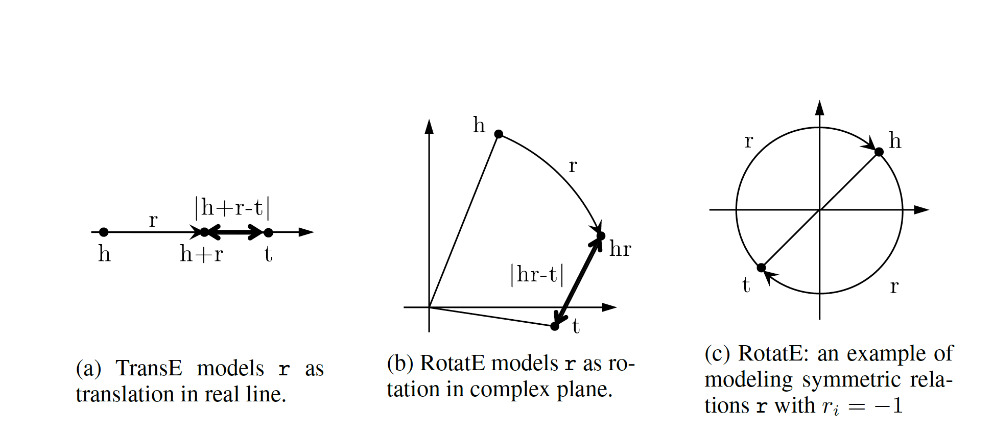
Score Function

score function of RotateE measures the angular distance between head and tail elements and is defined as:

$d_r(h, t)=\|h\circ r-t\|$

Training KE

Negative Sampling

Generally to train a KE, all the models we have investigated apply a variation of negative sampling by corrupting triplets $(h,r,t)$ . They corrupt either $h$ , or $t$ by sampling from set of head or tail entities for heads and tails respectively. The corrupted triples can be of wither forms $(h', r, t)$ or $(h, r, t')$ , where $h'$ and $t'$ are the negative samples.

Loss functions

Most commonly logistic loss and pairwise ranking loss are employed. The logistic loss returns -1 for negative samples and +1 for the positive samples. So if $\mathbb{D}^+$ and $\mathbb{D}^-$ are negative and positive data, $y=\pm 1$ is the label for positive and negative triplets and $f$ (figure 2) is the ranking function, then the logistic loss is computed as:

$minimize\ \sum_{(h,r,t)\in \mathbb{D}^+\cup \mathbb{D}^-}log(1+e^{-y\times f(h,r,t)})$

The second commonly use loss function is margin based pairwise ranking loss, which minimizes the rank for positive triplets( $(h,r,t)$ does hold). The lower the rank, the higher the probability. Ranking loss is give by:

$minimize \sum_{(h,r,t)\in \mathbb{D}^+}\sum_{(h,r,t)\in \mathbb{D}^-}max(0, \gamma - f(h,r,t)+f(h',r', t')).$

Method	Ent. Embedding	Rel. Emebedding	Score Function	Complexity	symm	Anti	Inv	Comp
TransE	$h,t \in \mathbb{R}^d$	$r \in \mathbb{R}^d$	$-\|\|h+r-t\|\|$	$O(d)$	$-$	$\checkmark$	$\checkmark$	$-$
TransR	$h,t \in \mathbb{R}^d$	$r \in \mathbb{R}^k,M_r\in\mathbb{R}^{k\times d}$	$-\|\|M_rh+r-M_rt\|\|_2^2$	$O(d^2)$	$-$	$\checkmark$	$\checkmark$	$\checkmark$
RESCAL	$h,t \in \mathbb{R}^d$	$M_r\in\mathbb{R}^{d\times d}$	$h^\top M_rt$	$O(d^2)$	$\checkmark$	$-$	$\checkmark$	$\checkmark$
DistMulti	$h,t \in \mathbb{R}^d$	$r\in\mathbb{R}^d$	$h^\top diag(r)t$	$O(d)$	$\checkmark$	$-$	$-$	$-$
ComplEx	$h,t \in \mathbb{C}^d$	$r\in\mathbb{C}^d$	$h^\top Re(diag(r)t)$	$O(d)$	$\checkmark$	$\checkmark$	$\checkmark$	$-$
RotateE	$h,t \in \mathbb{C}^d$	$r\in\mathbb{C}^d$	$\|\|h\circ r-t\|\|$	$O(d)$	$\checkmark$	$\checkmark$	$\checkmark$	$\checkmark$

References

http://semantic-web-journal.net/system/files/swj1167.pdf
Zhiqing Sun, Zhi-Hong Deng, Jian-Yun Nie, and Jian Tang. RotatE: Knowledge graph embedding by relational rotation in complex space. CoRR, abs/1902.10197, 2019.
Knowledge Graph Embedding: A Survey of Approaches and Applications Quan Wang, Zhendong Mao, Bin Wang, and Li Guo. DOI 10.1109/TKDE.2017.2754499, IEEE Transactions on Knowledge and Data Engineering
transE: Antoine Bordes, Nicolas Usunier, Alberto Garcia-Duran, JasonWeston, and Oksana Yakhnenko. Translating embeddings for modeling multi-relational data. In Advances in Neural Information Processing Systems 26. 2013. 5.TransR: Yankai Lin, Zhiyuan Liu, Maosong Sun, Yang Liu, and Xuan Zhu. Learning entity and relation embeddings for knowledge graph completion. In Proceedings of the Twenty-Ninth AAAI Conference on Artificial Intelligence, 2015.
RESCAL: Maximilian Nickel, Volker Tresp, and Hans-Peter Kriegel. A three-way model for collective learning on multi-relational data. In Proceedings of the 28th International Conference on International Conference on Machine Learning, ICML’11, 2011.
Survey paper: Q. Wang, Z. Mao, B. Wang and L. Guo, “Knowledge Graph Embedding: A Survey of Approaches and Applications,” in IEEE Transactions on Knowledge and Data Engineering, vol. 29, no. 12, pp. 2724-2743, 1 Dec. 2017.
DistMult: Bishan Yang, Scott Wen-tau Yih, Xiaodong He, Jianfeng Gao, and Li Deng. Embedding entities and relations for learning and inference in knowledge bases. In Proceedings of the International Conference on Learning Representations (ICLR) 2015, May 2015.
ComplEx: Théo Trouillon, Johannes Welbl, Sebastian Riedel, Éric Gaussier, and Guillaume Bouchard. Complex embeddings for simple link prediction. CoRR, abs/1606.06357, 2016.
Zhiqing Sun, Zhi-Hong Deng, Jian-Yun Nie, and Jian Tang. RotatE: Knowledge graph embedding by relational rotation in complex space. CoRR, abs/1902.10197, 2019.

DGL-KE Command Lines

原文档地址: https://dglke.dgl.ai/doc/commands.html .

DGL-KE provides a set of command line tools to train knowledge graph embeddings and make prediction with the embeddings easily.

Commands for Training

DGL-KE provides commands to support training on CPUs, GPUs in a single machine and a cluster of machines.

dglke_train trains KG embeddings on CPUs or GPUs in a single machine and saves the trained node embeddings and relation embeddings on disks.

dglke_dist_train trains knowledge graph embeddings on a cluster of machines. This command launches a set of processes to perform distributed training automatically.

To support distributed training, DGL-KE provides a command to partition a knowledge graph before training.

dglke_partition partitions the given knowledge graph into N parts by the METIS partition algorithm. Different partitions will be stored on different machines in distributed training. You can find more details about the METIS partition algorithm in this link.

In addition, DGL-kE provides a command to evaluate the quality of pre-trained embeddings.

dglke_eval reads the pre-trained embeddings and evaluates the quality of the embeddings with a link prediction task on the test set.

Commands for Inference

DGL-KE supports two types of inference tasks using pretained embeddings (We recommand using DGL-KE to generate these embedding).

Predicting entities/relations in a triplet Given entities and/or relations, predict which entities or relations are likely to connect with the existing entities for given relations. For example, given a head entity and a relation, predict which entities are likely to connect to the head entity via the given relation.
Finding similar embeddings Given entity/relation embeddings, find the most similar entity/relation embeddings for some pre-defined similarity functions.

The ranking result will be automatically stored in the output file (result.tsv by default) using the tsv format. DGL-KE provides two commands for the inference tasks:

dglke_predict predicts missing entities/relations in triplets using the pre-trained embeddings.
dglke_emb_sim computes similarity scores on the entity embeddings or relation embeddings.

Format of Input Data

原文档地址: https://dglke.dgl.ai/doc/format_kg.html .

DGL-KE toolkits provide commands for training, evaluation and inference. Different commands require different kinds of input data, including:

Knowledge Graph The knowledge graph used in train, evaluation and inference.
Trained Embeddings The embedding generated by dglke_train or dglke_dist_train.
Other Data Extra input data that used by inference tools.

A knowledge graph is usually stored in the form of triplets (head, relation, tail). Heads and tails are entities in the knowledge graph. All of them can be identified with unique IDs. In general, there exists two types of IDs for entities and relations in DGL-KE:

Raw ID The entities and relations can be identified by names, usually in the format of strings.
KGE ID They are used during knowledge graph training, evaluation and inference. Both entities and relations are identified with integers and should start from 0 and be contiguous.

If the input file of a knowledge graph uses Raw IDs for entities and relations and does not provide a mapping between Raw IDs and KGE Ids, DGL-KE will generate an ID mapping automatically.

The following table gives the overview of the input data for different toolkits. (Y for necessary and N for no-usage)

DGL-KE Toolkit	Knowledge Graph		Trained Embeddings	Other Data
	Triplets	ID Mapping	Embeddings
dglke_train	Y	Y	N	N
dglke_eval	Y	N	Y	N
dglke_partition	Y	Y	N	N
dglke_dist_train	Use data generated by dglke_partition
dglke_predict	N	Y	Y	Y
dglke_emb_sim	N	Y	Y	Y

Format of Knowledge Graph Used by DGL-KE

DGL-KE support three kinds of Knowledge Graph Input:

Built-in Knowledge Graph Built-in knowledge graphs are preprocessed datasets provided by DGL-KE package. There are five built-in datasets: FB15k, FB15k-237, wn18, wn18rr, Freebase.
Raw User Defined Knowledge Graph Raw user defined knowledge graph dataset uses the Raw IDs. Necessary ID convertion is needed before training a KGE model on the dataset. dglke_train, dglke_eval and dglke_partition provides the basic ability to do the ID convertion automatically.
KGE User Defined Knowledge Graph KGE user defined knowledge graph dataset already uses KGE IDs. The entities and relations in triplets are integers.

Format of Built-in Knowledge Graph

DGL-KE provides five built-in knowledge graphs:

Dataset	nodes	edges	relations
FB15k	14,951	592,213	1,345
FB15k-237	14,541	310,116	237
wn18	40,943	151,442	18
wn18rr	40,943	93,003	11
Freebase	86,054,151	338,586,276	14,824

Each of these built-in datasets contains five files:

train.txt: training set, each line contains a triplet [h, r, t]
valid.txt: validation set, each line contains a triplet [h, r, t]
test.txt: test set, each line contains a triplet [h, r, t]
entities.dict: ID mapping of entities
relations.dict: ID mapping of relations

Format of Raw User Defined Knowledge Graph

Raw user defined knowledge graph dataset uses the Raw IDs. The knowledge graph can be stored in a single file (only providing the trainset) or in three files (trainset, validset and testset). Each file stores the triplets of the knowledge graph. The order of head, relation and tail can be arbitry, e.g. [h, r, t]. A delimiter should be used to seperate them. The recommended delimiter includes \t, |, , and ;. The ID mapping is automatically generated by DGL-KE toolkits for raw user defined knowledge graphs.

Following gives an example of Raw User Defined Knowledge Graph files:

train.txt:

"Beijing","is_capital_of","China"
"Pairs","is_capital_of","France"
"London","is_capital_of","UK"
"UK","located_at","Europe"
"China","located_at","Asia"
"Tokyo","is_capital_of","Japan"

valid.txt:

1	"France","located_at","Europe"

test.txt:

1	"Japan","located_at","Asia"

Format of User Defined Knowledge Graph

User Defined Knowledge Graph uses the KGE IDs, which means both the entities and relations have already been remapped. The entity IDs and relation IDs are both start from 0 and be contiguous. The knowledge graph can be stored in a single file (only providing the trainset) or in three files (trainset, validset and testset) along with two ID mapping files (one for entity ID mapping and another for relation ID mapping). The knowledge graph is stored as triplets in files. The order of head, relation and tail can be arbitry, e.g. [h, r, t]. A delimiter should be used to seperate them. The recommended delimiter includes \t, |, , and ;. The ID mapping information is stored as pairs in mapping files with pair[0] as the integer ID and pair[1] as the original raw ID. The dglke_train and dglke_dist_train will do some integrity check of the IDs according to the mapping files.

Following gives an example of User Defined Knowledge Graph files:

train.txt:

0,0,1
2,0,3
4,0,5
5,1,6
1,1,7
8,0,9

valid.txt:

3,1,6

test.txt:

9,1,7

Following gives an example of entity ID mapping file:

entities.dict:

0,"Beijing"
1,"China"
2,"Pairs"
3,"France"
4,"London"
5,"UK"
6,"Europe"
7,"Asia"
8,"Tokyo"
9,"Japan"

Following gives an example of relation ID mapping file:

relations.dict:

1 2	0,"is_capital_of" 1,"located_at"

Format of Trained Embeddings

The trained embeddings are generated by dglke_train or dglke_dist_train CMD. The trained embeddings are stored in npy format. Usually there are two files:

Entity embeddings Entity embeddings are stored in a file named in format of dataset_name>_<model>_entity.npy and can be loaded through numpy.load().
Relation embeddings Relation embeddings are stored in a file named in format of dataset_name>_<model>_relation.npy and can be loaded through numpy.load().

Format of Input Data Used by DGL-KE Inference Tools

Both dglke_predict and dglke_emb_sim require user provied list of inferencing object.

Format of Raw Input Data

Raw Input Data uses the Raw IDs. Thus the input file contains objects in raw IDs and necessary ID mapping file(s) are required. Each line of the input file contains only one object and it can contains multiple lines. The ID mapping file store mapping information in pairs with pair[0] as the integer ID and pair[1] as the original raw ID.

Following gives an example of raw input files for dglke_predict:

head.list:

1 2	"Beijing" "London"

rel.list:

1	"is_capital_of"

tail.list:

1
2
3

"China"
"France"
"UK"

entities.dict:

0,"Beijing"
1,"China"
2,"Pairs"
3,"France"
4,"London"
5,"UK"
6,"Europe"

relations.dict:

1 2	0,"is_capital_of" 1,"located_at"

Format of KGE Input Data

KGE Input Data uses the KGE IDs. Thus the input file contains objects in KGE IDs, i.e., intergers. Each line of the input file contains only one object and it can contains multiple lines.

Following gives an example of raw input files for dglke_predict:

head.list:

1
2

0
4

rel.list:

tail.list:

1
2
3

1
3
5

Format of Output

原文档地址: https://dglke.dgl.ai/doc/format_out.html .

Different DGL-KE command line toolkits has different output data. Basically they have following dependency:

dglke_dist_train depends on the output of dglke_partition
dglke_eval depends on the output (Trained Embeddings) of the training CMD dglke_train or dglke_dist_train
dglke_predict and dglke_emb_sim depends on the the output (Trained Embeddings) of the training CMD dglke_train or dglke_dist_train as well as the ID mapping file.

Output format of dglke_partition

dglke_partition parititions a graph into parts. It generates N partition directories according to the input argument -k N. For example, when we set -k to 4, it will generate 4 directories: partition_0, partition_1, partition_2, and partition_3.

The detailed format of each partition_n is used by dglke_dist_train only and is out of the current scope. Please refer to distributed train section for more details.

Output format of dglke_train and dglke_dist_train

The output of dglke_train and dglke_dist_train are almost the same. Here we explain the output of dglke_train in this paragraph.

Basically there are four outputs:

Trained Embeddings: The saved model. For most of models like TransE, RESCAL, DistMult, ComplEx, and RotatE, there will be two files: <dataset_name>_<model>_entity.npy for entity embedding and <dataset_name>_<model>_relation.npy for relation embedding. There are all saved numpy tensor objects. For TransR, there is one additional output for saving the projection matrix.
config.json: The config file records all the details of the training configurations as well as the locations of ID mapping files generated by dgl_train. The fields of the config file are shown below:

Field Name	Explanation
neg_sample_size	int value of param –neg_sample_size
max_train_step	int value of param –max_step
double_ent	bool value of param –double_ent
rmap_file	relation ID mapping file name
lr	float value of param –lr
neg_adversarial_sampling	bool value of param –neg_adversarial_sampling
gamma	float value of param – gamma
adversarial_temperature	float value of param – adversarial_temperature
batch_size	int value of param – batch_size
regularization_coef	float value of param –regularization_coef
model	model name
dataset	dataset name
emb_size	embedding dimention size
regularization_norm	int value of param –regularization_norm
double_rel	bool value of param –double_rel
emap_file	entity ID mapping file name

Training Log: The output log printed to stdout. If --test is set. The final test result is also output (MR, MRR, Hit@1, Hit@3, Hit@10).
ID mapping Files (Optional): The the input data is in format of Raw User Defined Knowledge Graph, that is all triplets use the Raw ID space. The training script will do the ID convertion and generate two ID mapping files:
- entities.tsv, for entity ID mapping in format of KGE_entity_ID\tRaw_entity_Name, for example:
1
2
0\tBeijing
1\tChina
- relations.tsv, for relation ID mapping in format of KGE_relation_ID\tRaw_relation_name, for example:
1
2
0\tis_capital_of
1\tlocated_at

Output format of dglke_eval

There will be only one output of dglke_eval, the testing result including MR, MRR, Hit@1, Hit@3, Hit@10.

Output format of dglke_predict

The output of dglke_predict is a list of top ranked candidate (h, r, t) triplets as well as their prediction scores. The output is by default written into result.tsv and in the format of src\trel\tdst\tscore.

The example output is as:

src  rel  dst  score
6    0    15   -2.39380
8    0    14   -2.65297
2    0    14   -2.67331
9    0    18   -2.86985
8    0    20   -2.89651

If the input data of dglke_predict is in Raw IDs, dglke_predict will also convert the output result in Raw IDs.

Output format of dglke_emb_sim

The output of dglke_emb_sim is a list of top ranked candidate (left, right) pairs as well as their embedding similarity scores. The output is by default written into result.tsv and in the format of left\tright\tscore.

The example output is as:

left    right   score
6       15      0.55512
1       12      0.33153
7       20      0.27706
7       19      0.25631
7       13      0.21372

If the input data of dglke_emb_sim is in Raw IDs, dglke_emb_sim will also convert the output result in Raw IDs.

The example output is as:

left                          right                           score
_hyponym                      _hyponym                        0.99999
_derivationally_related_form  _derivationally_related_form    0.99999
_hyponym                      _also_see                       0.58408
_hyponym                      _member_of_domain_topic         0.44027
_hyponym                      _member_of_domain_region        0.30975

Training in a single machine

原文档地址: https://dglke.dgl.ai/doc/train.html .

dglke_train trains KG embeddings on CPUs or GPUs in a single machine and saves the trained node embeddings and relation embeddings on disks.

Arguments

The command line provides the following arguments:

--model_name {TransE, TransE_l1, TransE_l2, TransR, RESCAL, DistMult, ComplEx, RotatE} The models provided by DGL-KE.
--data_path DATA_PATH The path of the directory where DGL-KE loads knowledge graph data.
--dataset DATA_SET The name of the knowledge graph stored under data_path. If it is one of the builtin knowledge grpahs such as FB15k, FB15k-237, wn18, wn18rr, and Freebase, DGL-KE will automatically download the knowledge graph and keep it under data_path.
--format FORMAT The format of the dataset. For builtin knowledge graphs, the format is determined automatically. For users own knowledge graphs, it needs to be raw_udd_{htr} or udd_{htr}. raw_udd_ indicates that the user’s data use raw ID for entities and relations and udd_ indicates that the user’s data uses KGE ID. {htr} indicates the location of the head entity, tail entity and relation in a triplet. For example, htr means the head entity is the first element in the triplet, the tail entity is the second element and the relation is the last element.
--data_files [DATA_FILES ...] A list of data file names. This is required for training KGE on their own datasets. If the format is raw_udd_{htr}, users need to provide train_file [valid_file] [test_file]. If the format is udd_{htr}, users need to provide entity_file relation_file train_file [valid_file] [test_file]. In both cases, valid_file and test_file are optional.
--delimiter DELIMITER Delimiter used in data files. Note all files should use the same delimiter.
--save_path SAVE_PATH The path of the directory where models and logs are saved.
--no_save_emb Disable saving the embeddings under save_path.
--max_step MAX_STEP The maximal number of steps to train the model in a single process. A step trains the model with a batch of data. In the case of multiprocessing training, the total number of training steps is MAX_STEP * NUM_PROC.
--batch_size BATCH_SIZE The batch size for training.
--batch_size_eval BATCH_SIZE_EVAL The batch size used for validation and test.
--neg_sample_size NEG_SAMPLE_SIZE The number of negative samples we use for each positive sample in the training.
--neg_deg_sample Construct negative samples proportional to vertex degree in the training. When this option is turned on, the number of negative samples per positive edge will be doubled. Half of the negative samples are generated uniformly while the other half are generated proportional to vertex degree.
--neg_deg_sample_eval Construct negative samples proportional to vertex degree in the evaluation.
--neg_sample_size_eval NEG_SAMPLE_SIZE_EVAL The number of negative samples we use to evaluate a positive sample.
--eval_percent EVAL_PERCENT Randomly sample some percentage of edges for evaluation.
--no_eval_filter Disable filter positive edges from randomly constructed negative edges for evaluation.
--log_interval LOG_INTERVAL Print runtime of different components every LOG_INTERVAL steps.
--eval_interval EVAL_INTERVAL Print evaluation results on the validation dataset every EVAL_INTERVAL steps if validation is turned on.
--test Evaluate the model on the test set after the model is trained.
--num_proc NUM_PROC The number of processes to train the model in parallel. In multi-GPU training, the number of processes by default is the number of GPUs. If it is specified explicitly, the number of processes needs to be divisible by the number of GPUs.
--num_thread NUM_THREAD The number of CPU threads to train the model in each process. This argument is used for multi-processing training.
--force_sync_interval FORCE_SYNC_INTERVAL We force a synchronization between processes every FORCE_SYNC_INTERVAL steps for multiprocessing training. This potentially stablizes the training process to get a better performance. For multiprocessing training, it is set to 1000 by default.
--hidden_dim HIDDEN_DIM The embedding size of relations and entities.
--lr LR The learning rate. DGL-KE uses Adagrad to optimize the model parameters.
-g GAMMA or --gamma GAMMA The margin value in the score function. It is used by TransX and RotatE.
-de or --double_ent Double entitiy dim for complex number It is used by RotatE.
-dr or --double_rel Double relation dim for complex number.
-adv or --neg_adversarial_sampling Indicate whether to use negative adversarial sampling. It will weight negative samples with higher scores more.
-a ADVERSARIAL_TEMPERATURE or --adversarial_temperature ADVERSARIAL_TEMPERATURE The temperature used for negative adversarial sampling.
-rc REGULARIZATION_COEF or --regularization_coef REGULARIZATION_COEF The coefficient for regularization.
-rn REGULARIZATION_NORM or --regularization_norm REGULARIZATION_NORM norm used in regularization.
--gpu [GPU ...] A list of gpu ids, e.g. 0 1 2 4
--mix_cpu_gpu Training a knowledge graph embedding model with both CPUs and GPUs.The embeddings are stored in CPU memory and the training is performed in GPUs.This is usually used for training large knowledge graph embeddings.
--valid Evaluate the model on the validation set in the training.
--rel_part Enable relation partitioning for multi-GPU training.
--async_update Allow asynchronous update on node embedding for multi-GPU training. This overlaps CPU and GPU computation to speed up.

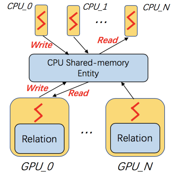
Training on Multi-Core

Multi-core processors are very common and widely used in modern computer architecture. DGL-KE is optimized on multi-core processors. In DGL-KE, we uses multi-processes instead of multi-threads for parallel training. In this design, the enity embeddings and relation embeddings will be stored in a global shared-memory and all the trainer processes can read and write it. All the processes will train the global model in a Hogwild style.

The following command trains the transE model on FB15k dataset on a multi-core machine. Note that, the total number of steps to train the model in this case is 24000:

1
2
3

dglke_train --model_name TransE_l2 --dataset FB15k --batch_size 1000 --neg_sample_size 200 --hidden_dim 400 \
--gamma 19.9 --lr 0.25 --max_step 3000 --log_interval 100 --batch_size_eval 16 --test -adv \
--regularization_coef 1.00E-09 --num_thread 1 --num_proc 8

After training, you will see the following messages:

-------------- Test result --------------
Test average MRR : 0.6520483281422476
Test average MR : 43.725415178344704
Test average HITS@1 : 0.5257063533713666
Test average HITS@3 : 0.7524081190431853
Test average HITS@10 : 0.8479202993008413
-----------------------------------------

Training on single GPU

Training knowledge graph embeddings requires a large number of tensor computation, which can be accelerated by GPU. DGL-KE can run on a single GPU, as well as a multi-GPU machine. Also, it can run in a mix-gpu-cpu setting, where the embedding data cannot fit in GPU memory.

The following command trains the transE model on FB15k on a single GPU:

1
2
3

dglke_train --model_name TransE_l2 --dataset FB15k --batch_size 1000 --log_interval 100 \
--neg_sample_size 200 --regularization_coef=1e-9 --hidden_dim 400 --gamma 19.9 \
--lr 0.25 --batch_size_eval 16 --test -adv --gpu 0 --max_step 24000

Most of the options here we have already seen in the previous section. The only difference is that we add --gpu 0 to indicate that we will use 1 GPU to train our model. Compared to the cpu training, every 100 steps only takes 0.72 seconds on the Nvidia v100 GPU, which is much faster than 8.9 second in CPU training:

[proc 0]sample: 0.165, forward: 0.282, backward: 0.217, update: 0.087
[proc 0][Train](1900/24000) average pos_loss: 0.32798981070518496
[proc 0][Train](1900/24000) average neg_loss: 0.45353577584028243
[proc 0][Train](1900/24000) average loss: 0.3907627931237221
[proc 0][Train](1900/24000) average regularization: 0.0012039361777715384
[proc 0][Train] 100 steps take 0.726 seconds
[proc 0]sample: 0.137, forward: 0.282, backward: 0.218, update: 0.087
[proc 0][Train](2000/24000) average pos_loss: 0.31407852172851564
[proc 0][Train](2000/24000) average neg_loss: 0.44177248477935793
[proc 0][Train](2000/24000) average loss: 0.3779255014657974
[proc 0][Train](2000/24000) average regularization: 0.0012163800827693194
[proc 0][Train] 100 steps take 0.760 seconds
[proc 0]sample: 0.171, forward: 0.282, backward: 0.218, update: 0.087
[proc 0][Train](2100/24000) average pos_loss: 0.309254549741745
[proc 0][Train](2100/24000) average neg_loss: 0.43288875490427015
[proc 0][Train](2100/24000) average loss: 0.37107165187597274
[proc 0][Train](2100/24000) average regularization: 0.0012251652684062719
[proc 0][Train] 100 steps take 0.726 seconds
[proc 0]sample: 0.136, forward: 0.283, backward: 0.219, update: 0.087
[proc 0][Train](2200/24000) average pos_loss: 0.3109792047739029
[proc 0][Train](2200/24000) average neg_loss: 0.4351910164952278
[proc 0][Train](2200/24000) average loss: 0.3730851110816002
[proc 0][Train](2200/24000) average regularization: 0.0012286945607047528
[proc 0][Train] 100 steps take 0.732 seconds

Mix CPU-GPU training

By default, DGL-KE keeps all node and relation embeddings in GPU memory for single-GPU training. It cannot train embeddings of large knowledge graphs because the capacity of GPU memory typically is much smaller than the CPU memory. So if your KG embedding is too large to fit in the GPU memory, you can use the mix_cpu_gpu training:

1
2
3

dglke_train --model_name TransE_l2 --dataset FB15k --batch_size 1000 --log_interval 100 \
--neg_sample_size 200 --regularization_coef=1e-9 --hidden_dim 400 --gamma 19.9 \
--lr 0.25 --batch_size_eval 16 --test -adv --gpu 0 --max_step 24000 --mix_cpu_gpu

The mix_cpu_gpu training keeps node and relation embeddings in CPU memory and performs batch computation in GPU. In this way, you can train very large KG embeddings as long as your cpu memory can handle it even though the training speed of mix_cpu_gpu training is slower than pure GPU training:

[proc 0][Train](8200/24000) average pos_loss: 0.2720812517404556
[proc 0][Train](8200/24000) average neg_loss: 0.4004567116498947
[proc 0][Train](8200/24000) average loss: 0.3362689846754074
[proc 0][Train](8200/24000) average regularization: 0.0014934110222384334
[proc 0][Train] 100 steps take 0.958 seconds
[proc 0]sample: 0.133, forward: 0.339, backward: 0.185, update: 0.301
[proc 0][Train](8300/24000) average pos_loss: 0.27434037417173385
[proc 0][Train](8300/24000) average neg_loss: 0.40289842933416364
[proc 0][Train](8300/24000) average loss: 0.33861940175294875
[proc 0][Train](8300/24000) average regularization: 0.001497904829448089
[proc 0][Train] 100 steps take 0.970 seconds
[proc 0]sample: 0.145, forward: 0.339, backward: 0.185, update: 0.300
[proc 0][Train](8400/24000) average pos_loss: 0.27482498317956927
[proc 0][Train](8400/24000) average neg_loss: 0.40262984931468965
[proc 0][Train](8400/24000) average loss: 0.3387274172902107
[proc 0][Train](8400/24000) average regularization: 0.0015005254035349936
[proc 0][Train] 100 steps take 0.958 seconds
[proc 0]sample: 0.132, forward: 0.338, backward: 0.185, update: 0.301

As we can see, the mix_cpu_gpu training takes 0.95 seconds on every 100 steps. It is slower than pure GPU training (0.73) but still much faster than CPU (8.9).

Users can speed up the mix_cpu_gpu training by using --async_update option. When using this option, the GPU device will not wait for the CPU to finish its job when it performs update operation:

1
2
3

dglke_train --model_name TransE_l2 --dataset FB15k --batch_size 1000 --log_interval 100 \
--neg_sample_size 200 --regularization_coef=1e-9 --hidden_dim 400 --gamma 19.9 \
--lr 0.25 --batch_size_eval 16 --test -adv --gpu 0 --max_step 24000 --mix_cpu_gpu --async_update

We can see that the training time goes down from 0.95 to 0.84 seconds on every 100 steps:

[proc 0][Train](22500/24000) average pos_loss: 0.2683987358212471
[proc 0][Train](22500/24000) average neg_loss: 0.3919999450445175
[proc 0][Train](22500/24000) average loss: 0.33019934087991715
[proc 0][Train](22500/24000) average regularization: 0.0017611468932591378
[proc 0][Train] 100 steps take 0.842 seconds
[proc 0]sample: 0.161, forward: 0.381, backward: 0.200, update: 0.099
[proc 0][Train](22600/24000) average pos_loss: 0.2682730385661125
[proc 0][Train](22600/24000) average neg_loss: 0.39290413081645964
[proc 0][Train](22600/24000) average loss: 0.3305885857343674
[proc 0][Train](22600/24000) average regularization: 0.0017612565110903234
[proc 0][Train] 100 steps take 0.838 seconds
[proc 0]sample: 0.159, forward: 0.379, backward: 0.200, update: 0.098
[proc 0][Train](22700/24000) average pos_loss: 0.2688949206471443
[proc 0][Train](22700/24000) average neg_loss: 0.3927029174566269
[proc 0][Train](22700/24000) average loss: 0.33079892098903657
[proc 0][Train](22700/24000) average regularization: 0.0017607113404665142
[proc 0][Train] 100 steps take 0.859 seconds

Training on Multi-GPU

DGL-KE also supports multi-GPU training to accelerate training. The following figure depicts 4 GPUs on a single machine and connected to the CPU through a PCIe switch. Multi-GPU training automatically keeps node and relation embeddings on CPUs and dispatch batches to different GPUs.

The following command shows how to training our transE model using 4 Nvidia v100 GPUs jointly:

1
2
3

dglke_train --model_name TransE_l2 --dataset FB15k --batch_size 1000 --log_interval 1000 \
--neg_sample_size 200 --regularization_coef=1e-9 --hidden_dim 400 --gamma 19.9 \
--lr 0.25 --batch_size_eval 16 --test -adv --gpu 0 1 2 3 --max_step 6000 --async_update

Compared to single-GPU training, we change --gpu 0 to --gpu 0 1 2 3, and also we change --max_step from 24000 to 6000:

[proc 0][Train](5800/6000) average pos_loss: 0.2675808426737785
[proc 0][Train](5800/6000) average neg_loss: 0.3915132364630699
[proc 0][Train](5800/6000) average loss: 0.3295470401644707
[proc 0][Train](5800/6000) average regularization: 0.0017635633377358318
[proc 0][Train] 100 steps take 1.123 seconds
[proc 0]sample: 0.237, forward: 0.472, backward: 0.215, update: 0.198
[proc 3][Train](5800/6000) average pos_loss: 0.26807423621416093
[proc 3][Train](5800/6000) average neg_loss: 0.3898271417617798
[proc 3][Train](5800/6000) average loss: 0.32895069003105165
[proc 3][Train](5800/6000) average regularization: 0.0017631534475367515
[proc 3][Train] 100 steps take 1.157 seconds
[proc 3]sample: 0.248, forward: 0.489, backward: 0.217, update: 0.202
[proc 1][Train](5900/6000) average pos_loss: 0.267591707110405
[proc 1][Train](5900/6000) average neg_loss: 0.3929813900589943
[proc 1][Train](5900/6000) average loss: 0.3302865487337112
[proc 1][Train](5900/6000) average regularization: 0.0017678673949558287
[proc 1][Train] 100 steps take 1.140 seconds

As we can see, using 4 GPUs we have almost 3x end-to-end performance speedup.

Note that --async_update can increase system performance but it could also slow down the model convergence. So DGL-KE provides another option called --force_sync_interval that forces all GPU sync their model on every N steps. For example, the following command will sync model across GPUs on every 1000 steps:

1
2
3

dglke_train --model_name TransE_l2 --dataset FB15k --batch_size 1000 --log_interval 1000 \
--neg_sample_size 200 --regularization_coef=1e-9 --hidden_dim 400 --gamma 19.9 \
--lr 0.25 --batch_size_eval 16 --test -adv --gpu 0 1 2 3 --async_update --max_step 6000 --force_sync_interval 1000

Save embeddings

By default, dglke_train saves the embeddings in the ckpts folder. Each run creates a new folder in ckpts to store the training results. The new folder is named after xxxx_yyyy_zz, where xxxx is the model name, yyyy is the dataset name, zz is a sequence number that ensures a unique name for each run.

The saved embeddings are stored as numpy ndarrays. The node embedding is saved as XXX_YYY_entity.npy. The relation embedding is saved as XXX_YYY_relation.npy. XXX is the dataset name and YYY is the model name.

A user can disable saving embeddings with --no_save_emb. This might be useful for some cases, such as hyperparameter tuning.

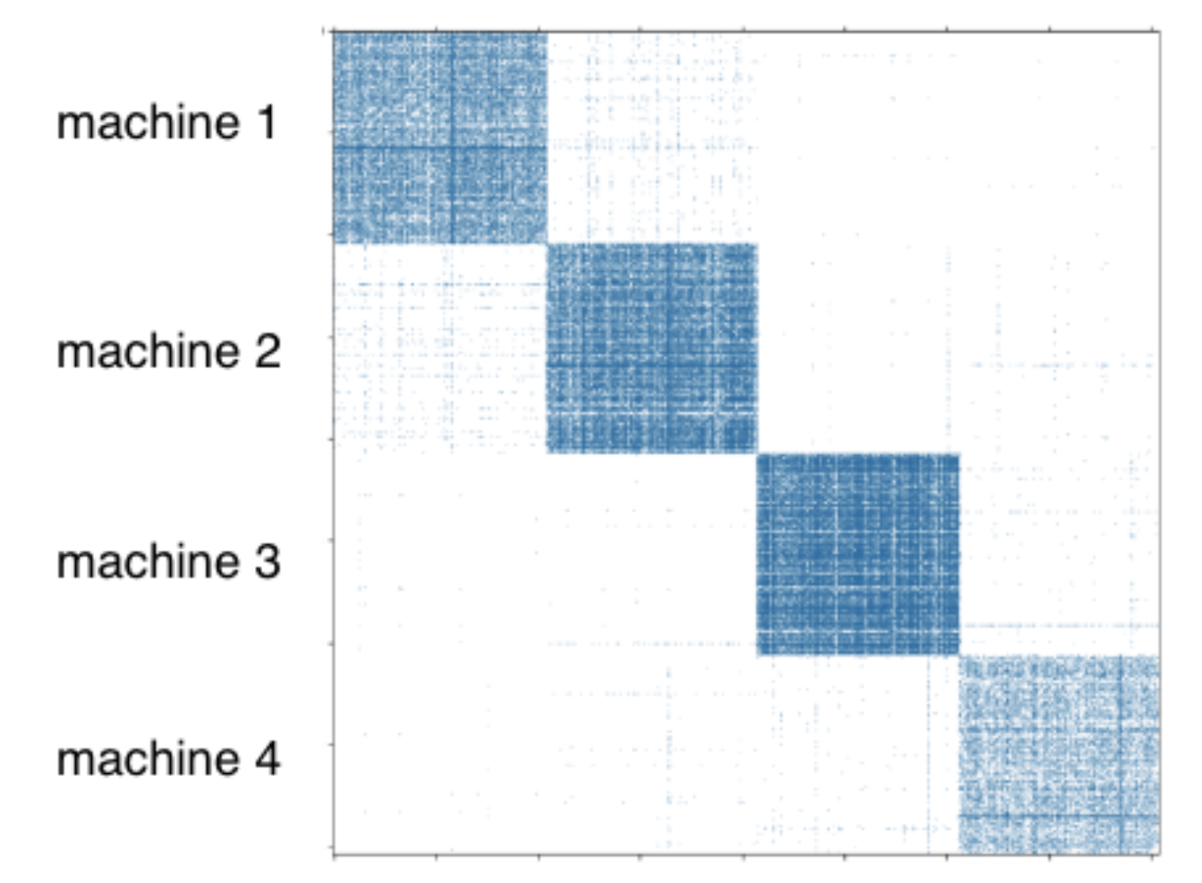
Partition a Knowledge Graph

原文档地址: https://dglke.dgl.ai/doc/partition.html .

For distributed training, a user needs to partition a graph beforehand. DGL-KE provides a partition tool dglke_partition, which partitions a given knowledge graph into N parts with the METIS partition algorithm. This partition algorithm reduces the number of edge cuts between partitions to reduce network communication in the distributed training. For a cluster of P machines, we usually split a graph into P partitions and assign a partition to a machine as shown in the figure below.

Arguments

The command line provides the following arguments:

--data_path DATA_PATH The name of the knowledge graph stored under data_path. If it is one ofthe builtin knowledge grpahs such as FB15k, DGL-KE will automatically download the knowledge graph and keep it under data_path.
--dataset DATA_SET The name of the knowledge graph stored under data_path. If it is one of the builtin knowledge grpahs such as FB15k, FB15k-237, wn18, wn18rr, and Freebase, DGL-KE will automatically download the knowledge graph and keep it under data_path.
--format FORMAT The format of the dataset. For builtin knowledge graphs, the format is determined automatically. For users own knowledge graphs, it needs to be raw_udd_{htr} or udd_{htr}. raw_udd_ indicates that the user’s data use raw ID for entities and relations and udd_ indicates that the user’s data uses KGE ID. {htr} indicates the location of the head entity, tail entity and relation in a triplet. For example, htr means the head entity is the first element in the triplet, the tail entity is the second element and the relation is the last element.
--data_files [DATA_FILES ...] A list of data file names. This is required for training KGE on their own datasets. If the format is raw_udd_{htr}, users need to provide train_file [valid_file] [test_file]. If the format is udd_{htr}, users need to provide entity_file relation_file train_file [valid_file] [test_file]. In both cases, valid_file and test_file are optional.
--delimiter DELIMITER Delimiter used in data files. Note all files should use the same delimiter.
-k NUM_PARTS or --num-parts NUM_PARTS The number of partitions.

Distributed Training on Large Data

原文档地址: https://dglke.dgl.ai/doc/dist_train.html .

dglke_dist_train trains knowledge graph embeddings on a cluster of machines. DGL-KE adopts the parameter-server architecture for distributed training.

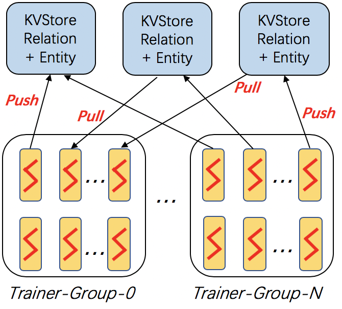
In this architecture, the entity embeddings and relation embeddings are stored in DGL KVStore. The trainer processes pull the latest model from KVStore and push the calculated gradient to the KVStore to update the model. All the processes trains the KG embeddings with asynchronous SGD.

Arguments

The command line provides the following arguments:

--model_name {TransE, TransE_l1, TransE_l2, TransR, RESCAL, DistMult, ComplEx, RotatE} The models provided by DGL-KE.
--data_path DATA_PATH The path of the directory where DGL-KE loads knowledge graph data.
--dataset DATA_SET The name of the knowledge graph stored under data_path. The knowledge graph should be generated by Partition script.
--format FORMAT The format of the dataset. For builtin knowledge graphs,the foramt should be built_in. For users own knowledge graphs,it needs to be raw_udd_{htr} or udd_{htr}.
--save_path SAVE_PATH The path of the directory where models and logs are saved.
--no_save_emb Disable saving the embeddings under save_path.
--max_step MAX_STEP The maximal number of steps to train the model in a single process. A step trains the model with a batch of data. In the case of multiprocessing training, the total number of training steps is MAX_STEP * NUM_PROC.
--batch_size BATCH_SIZE The batch size for training.
--batch_size_eval BATCH_SIZE_EVAL The batch size used for validation and test.
--neg_sample_size NEG_SAMPLE_SIZE The number of negative samples we use for each positive sample in the training.
--neg_deg_sample Construct negative samples proportional to vertex degree in the training. When this option is turned on, the number of negative samples per positive edge will be doubled. Half of the negative samples are generated uniformly whilethe other half are generated proportional to vertex degree.
--neg_deg_sample_eval Construct negative samples proportional to vertex degree in the evaluation.
--neg_sample_size_eval NEG_SAMPLE_SIZE_EVAL The number of negative samples we use to evaluate a positive sample.
--eval_percent EVAL_PERCENT Randomly sample some percentage of edges for evaluation.
--no_eval_filter Disable filter positive edges from randomly constructed negative edges for evaluation.
-log LOG_INTERVAL Print runtime of different components every x steps.
--test Evaluate the model on the test set after the model is trained.
--num_proc NUM_PROC The number of processes to train the model in parallel.
--num_thread NUM_THREAD The number of CPU threads to train the model in each process. This argument is used for multi-processing training.
--force_sync_interval FORCE_SYNC_INTERVAL We force a synchronization between processes every x steps formultiprocessing training. This potentially stablizes the training processto get a better performance. For multiprocessing training, it is set to 1000 by default.
--hidden_dim HIDDEN_DIM The embedding size of relation and entity.
--lr LR The learning rate. DGL-KE uses Adagrad to optimize the model parameters.
-g GAMMA or --gamma GAMMA The margin value in the score function. It is used by TransX and RotatE.
-de or --double_ent Double entitiy dim for complex number It is used by RotatE.
-dr or --double_rel Double relation dim for complex number.
-adv or --neg_adversarial_sampling Indicate whether to use negative adversarial sampling.It will weight negative samples with higher scores more.
-a ADVERSARIAL_TEMPERATURE or --adversarial_temperature ADVERSARIAL_TEMPERATURE The temperature used for negative adversarial sampling.
-rc REGULARIZATION_COEF or --regularization_coef REGULARIZATION_COEF The coefficient for regularization.
-rn REGULARIZATION_NORM or --regularization_norm REGULARIZATION_NORM norm used in regularization.
--path PATH Path of distributed workspace.
--ssh_key SSH_KEY ssh private key.
--ip_config IP_CONFIG Path of IP configuration file.
--num_client_proc NUM_CLIENT_PROC Number of worker processes on each machine.

The Steps for Distributed Training

Distributed training on DGL-KE usually involves three steps:

Partition a knowledge graph.
Copy partitioned data to remote machines.
Invoke the distributed training job by dglke_dist_train.

Here we demonstrate how to training KG embedding on FB15k dataset using 4 machines. Note that, the FB15k is just a small dataset as our toy demo. An interested user can try it on Freebase, which contains 86M nodes and 338M edges.

Step 1: Prepare your machines

Assume that we have four machines with the following IP addresses:

machine_0: 172.31.24.245
machine_1: 172.31.24.246
machine_2: 172.31.24.247
machine_3: 172.32.24.248

Make sure that machine_0 has the permission to ssh to all the other machines.

Step 2: Prepare your data

Create a new directory called my_task on machine_0:

1	mkdir my_task

We use built-in FB15k as demo and paritition it into 4 parts:

1	dglke_partition --dataset FB15k -k 4 --data_path ~/my_task

Note that, in this demo, we have 4 machines so we set -k to 4. After this step, we can see 4 new directories called partition_0, partition_1, partition_2, and partition_3 in your FB15k dataset folder.

Create a new file called ip_config.txt in my_task, and write the following contents into it:

172.31.24.245 30050 8
172.31.24.246 30050 8
172.31.24.247 30050 8
172.32.24.248 30050 8

Each line in ip_config.txt is the KVStore configuration on each machine. For example, 172.31.24.245 30050 8 represents that, on machine_0, the IP is 172.31.24.245, the base port is 30050, and we start 8 servers on this machine. Note that, you can change the number of servers on each machine based on your machine capabilities. In our environment, the instance has 48 cores, and we set 8 cores to KVStore and 40 cores for worker processes.

After that, we can copy the my_task directory to all the remote machines:

1
2
3

scp -r ~/my_task 172.31.24.246:~
scp -r ~/my_task 172.31.24.247:~
scp -r ~/my_task 172.31.24.248:~

Step 3: Launch distributed jobs

Run the following command on machine_0 to start a distributed task:

dglke_dist_train --path ~/my_task --ip_config ~/my_task/ip_config.txt \
--num_client_proc 16 --model_name TransE_l2 --dataset FB15k --data_path ~/my_task --hidden_dim 400 \
--gamma 19.9 --lr 0.25 --batch_size 1000 --neg_sample_size 200 --max_step 500 --log_interval 100 \
--batch_size_eval 16 --test -adv --regularization_coef 1.00E-09 --num_thread 1

Most of the options we have already seen in previous sections. Here are some new options we need to know.

--path indicates the absolute path of our workspace. All the logs and trained embedding will be stored in this path.
--ip_config is the absolute path of ip_config.txt.
--num_client_proc has the same behaviors to --num_proc in single-machine training.

All the other options are the same as single-machine training. For some EC2 users, you can also set --ssh_key for right ssh permission.

If you don’t set --no_save_embed option. The trained KG embeddings will be stored in machine_0/my_task/ckpts by default.

Evaluation on Pre-Trained Embeddings

原文档地址: https://dglke.dgl.ai/doc/eval.html .

dglke_eval reads the pre-trained embeddings and evaluates the quality of the embeddings with a link prediction task on the test set.

Arguments

The command line provides the following arguments:

--model_name {TransE, TransE_l1, TransE_l2, TransR, RESCAL, DistMult, ComplEx, RotatE} The models provided by DGL-KE.
--data_path DATA_PATH The name of the knowledge graph stored under data_path. If it is one ofthe builtin knowledge grpahs such as FB15k, DGL-KE will automatically download the knowledge graph and keep it under data_path.
--dataset DATASET The name of the knowledge graph stored under data_path. If it is one ofthe builtin knowledge grpahs such as FB15k, DGL-KE will automatically download the knowledge graph and keep it under data_path.
--format FORMAT The format of the dataset. For builtin knowledge graphs, the format is determined automatically. For users own knowledge graphs, it needs to be raw_udd_{htr} or udd_{htr}. raw_udd_ indicates that the user’s data use raw ID for entities and relations and udd_ indicates that the user’s data uses KGE ID. {htr} indicates the location of the head entity, tail entity and relation in a triplet. For example, htr means the head entity is the first element in the triplet, the tail entity is the second element and the relation is the last element.
--data_files [DATA_FILES ...] A list of data file names. This is used if users want to train KGE on their own datasets. If the format is raw_udd_{htr}, users need to provide train_file [valid_file] [test_file]. If the format is udd_{htr}, users need to provide entity_file relation_file train_file [valid_file] [test_file]. In both cases, valid_file and test_file are optional.
--delimiter DELIMITER Delimiter used in data files. Note all files should use the same delimiter.
--model_path MODEL_PATH The place where models are saved.
--batch_size_eval BATCH_SIZE_EVAL Batch size used for eval and test
--neg_sample_size_eval NEG_SAMPLE_SIZE_EVAL Negative sampling size for testing
--neg_deg_sample_eval Negative sampling proportional to vertex degree for testing.
--hidden_dim HIDDEN_DIM Hidden dim used by relation and entity
-g GAMMA or --gamma GAMMA The margin value in the score function. It is used by TransX and RotatE.
--eval_percent EVAL_PERCENT Randomly sample some percentage of edges for evaluation.
--no_eval_filter Disable filter positive edges from randomly constructed negative edges for evaluation.
--gpu [GPU ...] A list of gpu ids, e.g. 0 1 2 4
--mix_cpu_gpu Training a knowledge graph embedding model with both CPUs and GPUs.The embeddings are stored in CPU memory and the training is performed in GPUs.This is usually used for training a large knowledge graph embeddings.
-de or --double_ent Double entitiy dim for complex number It is used by RotatE.
-dr or --double_rel Double relation dim for complex number.
--num_proc NUM_PROC The number of processes to train the model in parallel.In multi-GPU training, the number of processes by default is set to match the number of GPUs. If set explicitly, the number of processes needs to be divisible by the number of GPUs.
--num_thread NUM_THREAD The number of CPU threads to train the model in each process. This argument is used for multi-processing training.

Examples

The following command evaluates the pre-trained KG embedding on multi-cores:

1 2	dglke_eval --model_name TransE_l2 --dataset FB15k --hidden_dim 400 --gamma 19.9 --batch_size_eval 16 \ --num_thread 1 --num_proc 8 --model_path ~/my_task/ckpts/TransE_l2_FB15k_0/

We can also use GPUs in our evaluation tasks:

1 2	dglke_eval --model_name TransE_l2 --dataset FB15k --hidden_dim 400 --gamma 19.9 --batch_size_eval 16 \ --gpu 0 1 2 3 4 5 6 7 --model_path ~/my_task/ckpts/TransE_l2_FB15k_0/

Predict entities/relations in triplets

原文档地址: https://dglke.dgl.ai/doc/predict.html .

dglke_predict predicts missing entities or relations in a triplet. Blow shows an example that predicts top 5 most likely destination entities for every given source node and relation:

src  rel  dst   score
 1    0    12   -5.11393
 1    0    18   -6.10925
 1    0    13   -6.66778
 1    0    17   -6.81532
 1    0    19   -6.83329
 2    0    17   -5.09325
 2    0    18   -5.42972
 2    0    20   -5.61894
 2    0    12   -5.75848
 2    0    14   -5.94183

Currently, it supports six models: TransE_l1, TransE_l2, RESCAL, DistMult, ComplEx, and RotatE.

Arguments

Four arguments are required to provide basic information for predicting missing entities or relations:

--model_path, The path containing the pretrained model, including the embedding files (.npy) and a config.json containing the configuration of training the model.
--format, The format of the input data, specified in h_r_t. Ideally, user should provides three files, one for head entities, one for relations and one for tail entities. But we also allow users to use * to represent all of the entities or relations. For example, h_r_* requires users to provide files containing head entities and relation entities and use all entities as tail entities; *_*_t requires users to provide a single file containing tail entities and use all entities as head entities and all relations. The supported formats include h_r_t, h_r_*, h_*_t, *_r_t, h_*_*, *_r_*, *_*_t.
--data_files A list of data file names. This is used to provide necessary files containing the input data according to the format, e.g., for h_r_t, the three input files are required and they contain a list of head entities, a list of relations and a list of tail entities. For h_*_t, two files are required, which contain a list of head entities and a list of tail entities.
--raw_data, A flag indicates whether the input data specified by –data_files use the raw Ids or KGE Ids. If True, the input data uses Raw IDs and the command translates IDs according to ID mapping. If False, the data use KGE IDs. Default False.

Task related arguments:

--exec_mode, How to calculate scores for triplets and calculate topK. Default ‘all’.
- triplet_wise: head, relation and tail lists have the same length N, and we calculate the similarity triplet by triplet: result = topK([score(h_i, r_i, t_i) for i in N]), the result shape will be (K,).
- all: three lists of head, relation and tail ids are provided as H, R and T, and we calculate all possible combinations of all triplets (h_i, r_j, t_k): result = topK([[[score(h_i, r_j, t_k) for each h_i in H] for each r_j in R] for each t_k in T]), and find top K from the triplets
- batch_head: three lists of head, relation and tail ids are provided as H, R and T, and we calculate topK for each element in head: result = topK([[score(h_i, r_j, t_k) for each r_j in R] for each t_k in T]) for each h_i in H. It returns (sizeof(H) * K) triplets.
- batch_rel: three lists of head, relation and tail ids are provided as H, R and T, and we calculate topK for each element in relation: result = topK([[score(h_i, r_j, t_k) for each h_i in H] for each t_k in T]) for each r_j in R. It returns (sizeof® * K) triplets.
- batch_tail: three lists of head, relation and tail ids are provided as H, R and T, and we calculate topK for each element in tail: result = topK([[score(h_i, r_j, t_k) for each h_i in H] for each r_j in R]) for each t_k in T. It returns (sizeof(T) * K) triplets.
--topk, How many results are returned. Default: 10.
--score_func, What kind of score is used in ranking. Currently, we support two functions: none (score = $x$ ) and logsigmoid ( $score = log(sigmoid(x))$ ). Default: none.
--gpu, GPU device to use in inference. Default: -1 (CPU)

Input/Output related arguments:

--output, the output file to store the result. By default it is stored in result.tsv.
--entity_mfile, The entity ID mapping file. Required if Raw ID is used.
--rel_mfile, The relation ID mapping file. Required if Raw ID is used.

Examples

The following command predicts the K most likely relations and tail entities for each head entity in the list using a pretrained TransE_l2 model (–exec_mode ‘batch_head’). In this example, the candidate relations and the candidate tail entities are given by the user.:

# Using PyTorch Backend
dglke_predict --model_path ckpts/TransE_l2_wn18_0/ --format 'h_r_t' --data_files head.list rel.list tail.list --score_func logsigmoid --topK 5 --exec_mode 'batch_head'

# Using MXNet Backend
MXNET_ENGINE_TYPE=NaiveEngine DGLBACKEND=mxnet dglke_predict --model_path ckpts/TransE_l2_wn18_0/ --format 'h_r_t' --data_files head.list rel.list tail.list --score_func logsigmoid --topK 5  --exec_mode 'batch_head'

The output is as:

src  rel  dst  score
1    0    12   -5.11393
1    0    18   -6.10925
1    0    13   -6.66778
1    0    17   -6.81532
1    0    19   -6.83329
2    0    17   -5.09325
2    0    18   -5.42972
2    0    20   -5.61894
2    0    12   -5.75848
2    0    14   -5.94183
...

The following command finds the most likely combinations of head entities, relations and tail entities from the input lists using a pretrained DistMult model:

# Using PyTorch Backend
dglke_predict --model_path ckpts/DistMult_wn18_0/ --format 'h_r_t' --data_files head.list rel.list tail.list --score_func none --topK 5

# Using MXNet Backend
MXNET_ENGINE_TYPE=NaiveEngine DGLBACKEND=mxnet dglke_predict --model_path ckpts/DistMult_wn18_0/ --format 'h_r_t' --data_files head.list rel.list tail.list --score_func none --topK 5

The output is as:

src  rel  dst  score
6    0    15   -2.39380
8    0    14   -2.65297
2    0    14   -2.67331
9    0    18   -2.86985
8    0    20   -2.89651

The following command finds the most likely combinations of head entities, relations and tail entities from the input lists using a pretrained TransE_l2 model and uses Raw ID (turn on –raw_data):

# Using PyTorch Backend
dglke_predict --model_path ckpts/TransE_l2_wn18_0/ --format 'h_r_t' --data_files raw_head.list raw_rel.list raw_tail.list --topK 5 --raw_data --entity_mfile data/wn18/entities.dict --rel_mfile data/wn18/relations.dict

# Using MXNet Backend
MXNET_ENGINE_TYPE=NaiveEngine DGLBACKEND=mxnet dglke_predict --model_path ckpts/TransE_l2_wn18_0/ --format 'h_r_t' --data_files raw_head.list raw_rel.list raw_tail.list --topK 5 --raw_data --entity_mfile data/wn18/entities.dict --rel_mfile data/wn18/relations.dict

The output is as:

head      rel                           tail      score
08847694  _derivationally_related_form  09440400  -7.41088
08847694  _hyponym                      09440400  -8.99562
02537319  _derivationally_related_form  01490112  -9.08666
02537319  _hyponym                      01490112  -9.44877
00083809  _derivationally_related_form  05940414  -9.88155

Find similar embeddings

原文档地址: https://dglke.dgl.ai/doc/emb_sim.html .

dglke_emb_sim finds the most similar entity/relation embeddings for some pre-defined similarity functions given a set of entities or relations. An example of the output for top5 similar entities are as follows:

left     right    score
0        0        0.99999
0        18470    0.91855
0        2105     0.89916
0        13605    0.83187
0        36762    0.76978

Currently we support five different similarity functions: cosine, l2 distance, l1 distance, dot product and extended jaccard.

Arguments

Four arguments are required to provide basic information for finding similar embeddings:

--emb_file, The numpy file that contains the embeddings of all entities/relations in a knowledge graph.
--format, The format of the input objects (entities/relations).
- l_r: two list of objects are provided as left objects and right objects.
- l_*: one list of objects is provided as left objects and all objects in emb_file are right objects. This is to find most similar objects to the ones on the left.
- *_r: one list of objects is provided as right objects list and treat all objects in emb_file as left objects.
- *: all objects in the emb_file are both left objects and right objects. The option finds the most similar objects in the graph.
--data_files A list of data file names. It provides necessary files containing the requried data according to the format, e.g., for l_r, two files are required as left_data and right_data, while for l_*, one file is required as left_data, and for * this argument will be omited.
--raw_data, A flag indicates whether the data in data_files are raw IDs or KGE IDs. If True, the data are the Raw IDs and the command will map the raw IDs to KGE Ids automatically using the ID mapping file provided through --mfile. If False, the data are KGE IDs. Default: False.

Task related arguments:

--exec_mode, Indicate how to calculate scores for element pairs and calculate topK. Default: ‘all’
- pairwise: The same number (N) of left and right objects are provided. It calculates the similarity pair by pair: result = topK([score(l_i, r_i) for i in N]) and output the K most similar pairs.
- all: both left objects and right objects are provided as L and R. It calculates similarity scores of all possible combinations of (l_i, r_j): result = topK([[score(l_i, rj) for l_i in L] for r_j in R]), and outputs the K most similar pairs.
- batch_left: left objects and right objects are provided as L and R. It finds the K most similar objects from the right objects for each object in L: result = topK([score(l_i, r_j) for r_j in R]) for l_j in L. It outputs (len(L) * K) most similar pairs.
--topk, How many results are returned. Default: 10.
--sim_func, the function to define the similarity score between a pair of objects. It support five functions. Default: cosine
- cosine: use cosine similarity; score = $\frac{x \cdot y}{||x||_2||y||_2}$
- l2: use l2 similarity; score = $-||x - y||_2$
- l1: use l1 similarity; score = $-||x - y||_1$
- dot: use dot product similarity; score = $x \cdot y$
- ext_jaccard: use extended jaccard similarity. score = $\frac{x \cdot y}{||x||_{2}^{2} + ||y||_{2}^{2} - x \cdot y}$
--gpu, GPU device to use in inference. Default: -1 (CPU).

Input/Output related arguments:

--output, the output file that stores the result. By default it is stored in result.tsv.
--mfile, The ID mapping file.

Examples

The following command finds similar entities based on cosine distance:

# Using PyTorch Backend
dglke_emb_sim --emb_file ckpts/TransE_l2_wn18_0/wn18_TransE_l2_entity.npy --format 'l_r' --data_files head.list tail.list  --topK 5

# Using MXNet Backend
MXNET_ENGINE_TYPE=NaiveEngine DGLBACKEND=mxnet dglke_emb_sim --emb_file ckpts/TransE_l2_wn18_0/wn18_TransE_l2_entity.npy --format 'l_r' --data_files head.list tail.list --topK 5

The output is as:

left    right   score
6       15      0.55512
1       12      0.33153
7       20      0.27706
7       19      0.25631
7       13      0.21372

The following command finds topK most similar entities for each element on the left using l2 distance (–exec_mode batch_left):

# Using PyTorch Backend
dglke_emb_sim --emb_file ckpts/TransE_l2_wn18_0/wn18_TransE_l2_entity.npy --format 'l_*' --data_files head.list --sim_func l2 --topK 5 --exec_mode 'batch_left'

# Using MXNet Backend
MXNET_ENGINE_TYPE=NaiveEngine DGLBACKEND=mxnet dglke_emb_sim --emb_file ckpts/TransE_l2_wn18_0/wn18_TransE_l2_entity.npy --format 'l_*' --data_files head.list --sim_func l2 --topK 5 --exec_mode 'batch_left'

The output is as:

left    right   score
0       0       0.0
0       18470   3.1008
0       24408   3.1466
0       2105    3.3411
0       13605   4.1587
1       1       0.0
1       26231   4.9025
1       2617    5.0204
1       12672   5.2221
1       38633   5.3221
...

The following command finds similar relations using cosine distance and use Raw ID (turn on –raw_data):

# Using PyTorch Backend
dglke_emb_sim --mfile data/wn18/relations.dict --emb_file ckpts/TransE_l2_wn18_0/wn18_TransE_l2_relation.npy  --format 'l_*' --data_files raw_rel.list --topK 5 --raw_data

# Using MXNet Backend
MXNET_ENGINE_TYPE=NaiveEngine DGLBACKEND=mxnet dglke_emb_sim --mfile data/wn18/relations.dict --emb_file ckpts/TransE_l2_wn18_0/wn18_TransE_l2_relation.npy  --format 'l_*' --data_files raw_rel.list --topK 5 --raw_data

The output is as:

left                          right                           score
_hyponym                      _hyponym                        0.99999
_derivationally_related_form  _derivationally_related_form    0.99999
_hyponym                      _also_see                       0.58408
_hyponym                      _member_of_domain_topic         0.44027
_hyponym                      _member_of_domain_region        0.30975

Train User-Defined Knowledage Graphs

原文档地址: https://dglke.dgl.ai/doc/train_user_data.html .

Users can use DGL-KE to train embeddings on their own knowledge graphs. In this case, users need to use --data_path to specify the path to the knowledge graph dataset, --data_files to specify the triplets of a knowledge graph as well as node/relation ID mapping, --format to specify the input format of the knowledge graph.

The input format of users’ knowledge graphs

Users need to store all the data associated with a knowledge graph in the same directory. DGL-KE supports two knowledge graph input formats:

Raw user-defined knowledge graphs: user only needs to provide triplets, both entities and relations in the triplets can be arbitrary strings. The dataloader will automatically generate the id mappings for entities and relations in the triplets. An example of triplets:

	train.tsv
Beijing	is_capital_of	China
London	is_capital_of	UK
UK	located_at	Europe
…

User-defined knowledge graphs: user need to provide the id mapping for entities and relations as well as the triplets of the knowledge graph. The triplets should only contains entities ids and relation ids. Here we assume the both the entities ids and relation ids start from 0 and should be contineous. An example of mapping and triplets files:

entities.dict	relation.dict	train.tsv
Beijing 0	is_capital_of 0	0 0 2
London 1	located_at 1	1 0 3
China 2		3 1 4
UK 3
Europe 4

Using raw user-defined knowledge graph format

Users need to store all the data associated with a knowledge graph in the same directory. DGL-KE supports two knowledge graph input formats:

raw_udd_[h|r|t]: In this format, users only need to provide triplets and the dataloader generates the id mappings for entities and relations in the triplets. The dataloader outputs two files: entities.tsv for entity id mapping and relations.tsv for relation id mapping while loading data. The order of head, relation and tail entities are described in [h|r|t], for example, raw_udd_trh means the triplets are stored in the order of tail, relation and head. The directory contains three files:

train stores the triplets in the training set. The format of a triplet, e.g., [src_name, rel_name, dst_name], should follow the order specified in [h|r|t]
valid stores the triplets in the validation set. The format of a triplet, e.g., [src_name, rel_name, dst_name], should follow the order specified in [h|r|t]. This is optional.
test stores the triplets in the test set. The format of a triplet, e.g., [src_name, rel_name, dst_name], should follow the order specified in [h|r|t]. This is optional.

Using user-defined knowledge graph format

udd_[h|r|t]: In this format, user should provide the id mapping for entities and relations. The order of head, relation and tail entities are described in [h|r|t], for example, raw_udd_trh means the triplets are stored in the order of tail, relation and head. The directory should contains five files:

entities stores the mapping between entity name and entity Id
relations stores the mapping between relation name relation Id
train stores the triplets in the training set. The format of a triplet, e.g., [src_id, rel_id, dst_id], should follow the order specified in [h|r|t]
valid stores the triplets in the validation set. The format of a triplet, e.g., [src_id, rel_id, dst_id], should follow the order specified in [h|r|t]
test stores the triplets in the test set. The format of a triplet, e.g., [src_id, rel_id, dst_id], should follow the order specified in [h|r|t]

Benchmarks on Built-in Knowledage Graphs

原文档地址: https://dglke.dgl.ai/doc/benchmarks.html .

DGL-KE provides five built-in knowledge graphs:

Dataset	nodes	edges	relations
FB15k	14951	592213	1345
FB15k-237	14541	310116	237
wn18	40943	151442	18
wn18rr	40943	93003	11
Freebase	86054151	338586276	14824

Users can specify one of the datasets with --dataset option in their tasks.

DGL-KE provides benchmark results on FB15k, wn18, as well as Freebase. Users can go to the corresponded folder to check out the scripts and results. All the benchmark results are done by AWS EC2. For multi-cpu and distributed training, the target instance is r5dn.24xlarge, which has 48 CPU cores and 768 GB memory. Also, r5dn.xlarge has 100Gbit network throughput, which is powerful for distributed training. For GPU training, our target instance is p3.16xlarge, which has 64 CPU cores and 8 Nvidia v100 GPUs. For users, you can choose your own instance by your demand and tune the hyper-parameters for the best performance.

All the scripts can be found on this page.

FB15k

One-GPU training

Models	MR	MRR	HITS-1	HITS-3	HITS-10	TIME
TransE_l1	47.34	0.672	0.557	0.763	0.849	201
TransE_l2	47.04	0.649	0.525	0.746	0.844	167
DistMult	61.43	0.696	0.586	0.782	0.873	150
ComplEx	64.73	0.757	0.672	0.826	0.886	171
RESCAL	124.5	0.661	0.589	0.704	0.787	1252
TransR	59.99	0.670	0.585	0.728	0.808	530
RotatE	43.85	0.726	0.632	0.799	0.873	1405

8-GPU training

Models	MR	MRR	HITS-1	HITS-3	HITS-10	TIME
TransE_l1	48.59	0.662	0.542	0.756	0.846	53
TransE_l2	47.52	0.627	0.492	0.733	0.838	49
DistMult	59.44	0.679	0.566	0.764	0.864	47
ComplEx	64.98	0.750	0.668	0.814	0.883	49
RESCAL	133.3	0.643	0.570	0.685	0.773	179
TransR	66.51	0.666	0.581	0.724	0.803	90
RotatE	50.04	0.685	0.581	0.763	0.851	120

Multi-CPU training

Models	MR	MRR	HITS-1	HITS-3	HITS-10	TIME
TransE_l1	48.32	0.645	0.521	0.741	0.838	140
TransE_l2	45.28	0.633	0.501	0.735	0.840	58
DistMult	62.63	0.647	0.529	0.733	0.846	58
ComplEx	67.83	0.694	0.590	0.772	0.863	69

Distributed training

Models	MR	MRR	HITS-1	HITS-3	HITS-10	TIME
TransE_l1	38.26	0.691	0.591	0.765	0.853	104
TransE_l2	34.84	0.645	0.510	0.754	0.854	31
DistMult	51.85	0.661	0.532	0.762	0.864	57
ComplEx	62.52	0.667	0.567	0.737	0.836	65

wn18

One-GPU training

Models	MR	MRR	HITS-1	HITS-3	HITS-10	TIME
TransE_l1	355.4	0.764	0.602	0.928	0.949	327
TransE_l2	209.4	0.560	0.306	0.797	0.943	223
DistMult	419.0	0.813	0.702	0.921	0.948	133
ComplEx	318.2	0.932	0.914	0.948	0.959	144
RESCAL	563.6	0.848	0.792	0.898	0.928	308
TransR	432.8	0.609	0.452	0.736	0.850	906
RotatE	451.6	0.944	0.940	0.945	0.950	671

8-GPU training

Models	MR	MRR	HITS-1	HITS-3	HITS-10	TIME
TransE_l1	348.8	0.739	0.553	0.927	0.948	111
TransE_l2	198.9	0.559	0.305	0.798	0.942	71
DistMult	798.8	0.806	0.705	0.903	0.932	66
ComplEx	535.0	0.938	0.931	0.944	0.949	53
RotatE	487.7	0.943	0.939	0.945	0.951	127

Multi-CPU training

Models	MR	MRR	HITS-1	HITS-3	HITS-10	TIME
TransE_l1	376.3	0.593	0.264	0.926	0.949	925
TransE_l2	218.3	0.528	0.259	0.777	0.939	210
DistMult	837.4	0.791	0.675	0.904	0.933	362
ComplEx	806.3	0.904	0.881	0.926	0.937	281

Distributed training

Models	MR	MRR	HITS-1	HITS-3	HITS-10	TIME
TransE_l1	136.0	0.848	0.768	0.927	0.950	759
TransE_l2	85.04	0.797	0.672	0.921	0.958	144
DistMult	278.5	0.872	0.816	0.926	0.939	275
ComplEx	333.8	0.838	0.796	0.870	0.906	273

Freebase

8-GPU training

Models	MR	MRR	HITS-1	HITS-3	HITS-10	TIME
TransE_l2	23.56	0.736	0.663	0.782	0.873	4767
DistMult	46.19	0.833	0.813	0.842	0.869	4281
ComplEx	46.70	0.834	0.815	0.843	0.869	8356
TransR	49.68	0.696	0.653	0.716	0.773	14235
RotatE	93.20	0.769	0.748	0.779	0.804	9060

Multi-CPU training

Models	MR	MRR	HITS-1	HITS-3	HITS-10	TIME
TransE_l2	30.82	0.815	0.766	0.848	0.902	6993
DistMult	44.16	0.834	0.815	0.843	0.869	7146
ComplEx	45.62	0.835	0.817	0.843	0.870	8732

Distributed training

Models	MR	MRR	HITS-1	HITS-3	HITS-10	TIME
TransE_l2	34.25	0.764	0.705	0.802	0.869	1633
DistMult	75.15	0.769	0.751	0.779	0.801	1679
ComplEx	77.83	0.771	0.754	0.779	0.802	2293

Profile DGL-KE

原文档地址: https://dglke.dgl.ai/doc/profile.html .

This document is mainly for developing the DGL-KE models and accelerating their training.

To analyze MXNet version of KE models, please enable MXNet_PROFILER environment variable when running the training job:

1
2
3

MXNET_PROFILER=1 dglke_train --model_name TransE_l2 --dataset FB15k --batch_size 1000 --neg_sample_size 200 --hidden_dim 400 \
--gamma 19.9 --lr 0.25 --max_step 3000 --log_interval 100 --batch_size_eval 16 --test -adv \
--regularization_coef 1.00E-09 --num_thread 1 --num_proc 8