00032-人工智能杂项-ubuntu

前言

介绍一些人工智能杂项，包括：激活函数等问题。

操作系统：Ubuntu 20.04.4 LTS

参考文档

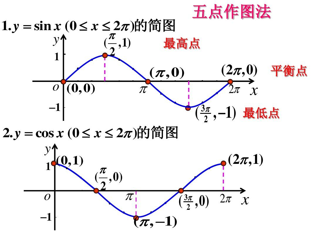
正余弦函数图像

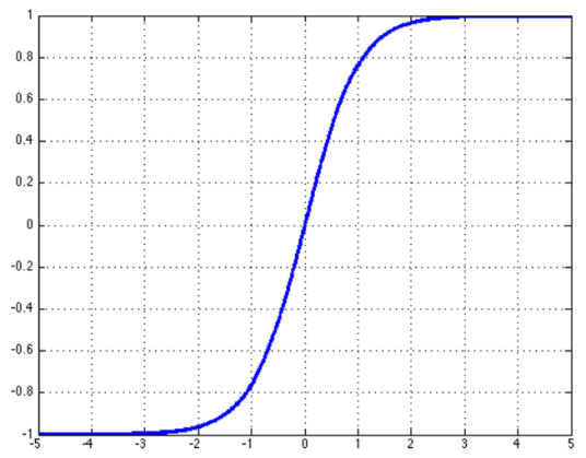
双曲正切函数

双曲正切函数（ $tanh$ ）是双曲正弦函数（ $sinh$ ）与双曲余弦函数（ $cosh$ ）的比值，其解析形式为：

$tanh x = \frac{sinh x}{cosh x} = \frac{e^x - e^{-x}}{e^x + e^{-x}}$

导数

$(tanh x)^{'} = sech^2x = \frac{1}{cosh^2x} = 1 - tanh^2x$

图像

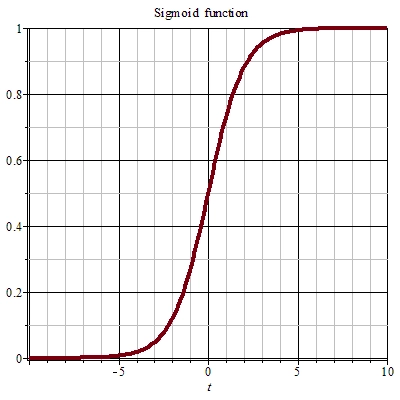
Sigmoid 函数

Sigmoid 函数也叫 Logistic 函数，其解析形式为：

$S(x) = \frac{1}{1 + e^{-x}}$

导数

$S^{'}(x) = \frac{e^{-x}}{(1 + e^{-x})^2} = S(x)(1 - S(x))$

图像

对数公式

$log_a(1) = 0$

$log_a(a) = 1$

$log_ab * log_ba = 1$

$-log_c\frac{a}{b} = log_c\frac{b}{a}$

$log_a(MN) = log_aM + log_aN$

$log_a(\frac{M}{N}) = log_aM - log_aN$

$log_a(\frac{1}{N}) = -log_aN$

$a^{log_ab} = b$

$log_aM^n = nlog_aM$

$log_a\sqrt[n]{M} = \frac{1}{n}log_aM$

$log_a(a^k) = k$

$log_ab = \frac{log_cb}{log_ca}$

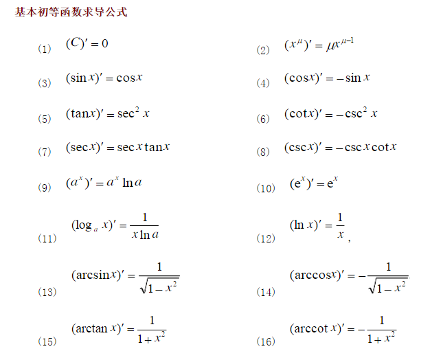
基本初等函数求导公式

更详细的求导公式可以参考: 导数表.

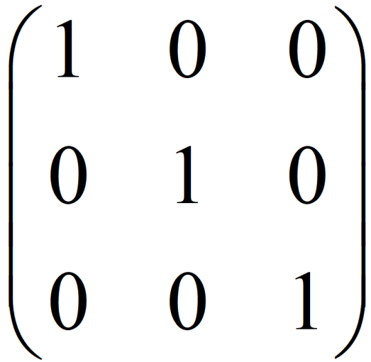
单位矩阵

源教程地址: https://baike.baidu.com/item/单位矩阵 .

在矩阵的乘法中，有一种矩阵起着特殊的作用，如同数的乘法中的1，这种矩阵被称为单位矩阵。它是个方阵，从左上角到右下角的对角线（称为主对角线）上的元素均为1。除此以外全都为0。

根据单位矩阵的特点，任何矩阵与单位矩阵相乘都等于本身，而且单位矩阵因此独特性在高等数学中也有广泛应用。

虚数 i 代表逆时针旋转 90 度

源教程地址: https://www.zhihu.com/question/412918345/answer/1534274299 .

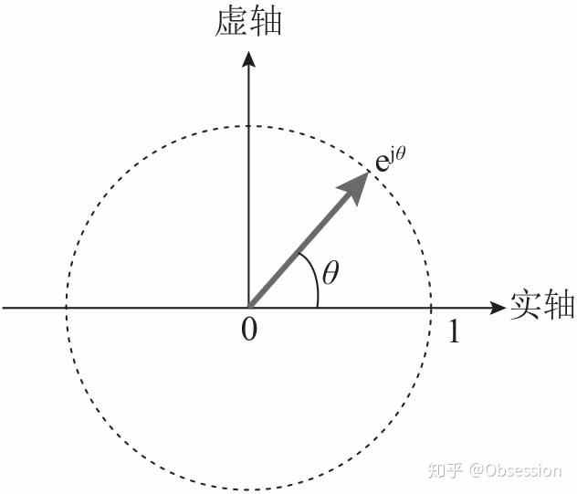
著名的欧拉公式：

$e^{j\theta}=cos\theta + jsin\theta$

$e^{j\theta}=cos\theta + jsin\theta$ 是一个复数，实部为 $cos\theta$ ，虚部为 $sin\theta$ ，在复平面上对应单位圆上的一个点。由欧拉公式，这个点可以用复指数表示，如图：

欧拉公式的证明:

下面用麦克劳林级数对欧拉公式进行证明：

$e^x=1+\frac{x}{1!}+\frac{x^2}{2!}+\frac{x^3}{3!}+\frac{x^4}{4!}+......$

用 $jx$ 替换 $x$ :

$e^{jx}=1+jx+\frac{(jx)^2}{2!}+\frac{(jx)^3}{3!}+\frac{(jx)^4}{4!}+\frac{(jx)^5}{5!}+\frac{(jx)^6}{6!}+\frac{(jx)^7}{7!}...\\ =1+jx-\frac{x^2}{2!}-j\frac{x^3}{3!}+\frac{x^4}{4!}+j\frac{x^5}{5!}-\frac{x^6}{6!}-j\frac{x^7}{7!}+...\\ =1-\frac{x^2}{2!}+\frac{x^4}{4!}-\frac{x^6}{6!}+...+j\lgroup x-\frac{x^3}{3!}+\frac{x^5}{5!}-\frac{x^7}{7!}+... \rgroup \\ =cosx+jsinx$

推导过程用到了 $cosx$ 和 $sinx$ 的麦克劳林展开式，证明完毕。

复数的几何意义:

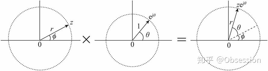
为了便于理解，通常用复平面上的向量来表示复数。复指数 $e^{j\theta}$ 对应的向量：始端为原点，长度为1，辐角为 $\theta$ .

引入向量之后，复数与复指数 $e^{j\theta}$ 相乘就可以用向量旋转来理解。

复数： $z=r(cos\varphi+jsin\varphi)$

直接套用欧拉公式，可得： $z=re^{j\varphi}$ ,复数z与复指数 $e^{j\varphi}$ 相乘：

$ze^{j\theta}=re^{j\varphi}e^{j\theta}=re^{j(\varphi + \theta)}$

也就是说：

复数与复指数 $e^{j\theta}$ 相乘，相当于复数对应的向量旋转角度 $\theta$ .

$\theta > 0$ , 逆时针旋转

$\theta < 0$ ，顺时针旋转

如图

如何理解虚数

复指数中引入了虚数 $j$ ，如何理解虚数 $j$ 呢？

数学中虚数一般用“i”来表示，物理中用“j”来表示，因为物理中已经用“i”来表示电流了。

关于虚数，如果追溯起来，在高中的时候我们就接触过了，当时只是给了一个概念， $i^2=-1$ 。按一般的理解，一个数和自己相乘，肯定是得到一个整数，负负得正么。

虚数刚被提出时，也曾困扰很多数学家，被大家认为是“虚无缥缈的数”，指导有了欧拉公式，人们才对虚数的物理意义有了清晰的认识。

下面我们一起来看看如何利用欧拉公式理解虚数。

在欧拉公式中，令 $\theta=\frac{\pi}{2}$ ，得：

$e^{j(\pi/2)=cos\pi/2+jsin\pi/2=j}$

即： $j=e^{j(\pi/2)}$

复数与 $j$ 相乘，就是与复指数 $e^{j(\pi/2)}$ 相乘，相当与复数逆时针旋转90度，也就是说，复数与 $j$ 相乘的过程，也就是向量旋转的过程，如图所示。

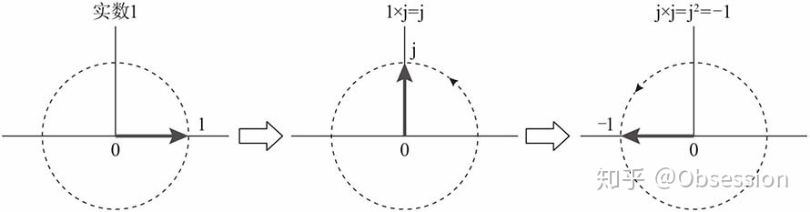
由前面的分析，进行总结：

实数1对应的向量逆时针旋转90度，得到虚数 $j$ ，即：

$1*j=j$

虚数 $j$ 对应的向量再逆时针旋转90度，得到实数-1，即：

$j*j=j^2=-1$

至此，通过一步步的推导，我们就可以对虚数j有一个清晰的认识啦。

傅里叶变换

教程: https://www.zhihu.com/question/19714540/answer/1119070975 .

NVIDIA Multi-Instance GPU

sklearn 常用的函数

euclidean_distances

文档链接: https://scikit-learn.org/stable/modules/generated/sklearn.metrics.pairwise.euclidean_distances.html#sklearn.metrics.pairwise.euclidean_distances .

sklearn.metrics.pairwise.euclidean_distances

sklearn.metrics.pairwise.euclidean_distances(X, Y=None, *, Y_norm_squared=None, squared=False, X_norm_squared=None)

Compute the distance matrix between each pair from a vector array X and Y.

For efficiency reasons, the euclidean distance between a pair of row vector x and y is computed as:

dist(x, y) = sqrt(dot(x, x) - 2 * dot(x, y) + dot(y, y))

This formulation has two advantages over other ways of computing distances. First, it is computationally efficient when dealing with sparse data. Second, if one argument varies but the other remains unchanged, then dot(x, x) and/or dot(y, y) can be pre-computed.

However, this is not the most precise way of doing this computation, because this equation potentially suffers from “catastrophic cancellation”. Also, the distance matrix returned by this function may not be exactly symmetric as required by, e.g., scipy.spatial.distance functions.

cosine_similarity

文档链接: https://scikit-learn.org/stable/modules/generated/sklearn.metrics.pairwise.cosine_similarity.html#sklearn.metrics.pairwise.cosine_similarity .

sklearn.metrics.pairwise.cosine_similarity

sklearn.metrics.pairwise.cosine_similarity(X, Y=None, dense_output=True)

Compute cosine similarity between samples in X and Y.

Cosine similarity, or the cosine kernel, computes similarity as the normalized dot product of X and Y:

K(X, Y) = <X, Y> / (||X||*||Y||)

On L2-normalized data, this function is equivalent to linear_kernel.

TSNE

文档链接: https://scikit-learn.org/stable/modules/generated/sklearn.manifold.TSNE.html#sklearn.manifold.TSNE .

sklearn.manifold.TSNE

class sklearn.manifold.TSNE(n_components=2, *, perplexity=30.0, early_exaggeration=12.0, learning_rate='auto', n_iter=1000, n_iter_without_progress=300, min_grad_norm=1e-07, metric='euclidean', metric_params=None, init='pca', verbose=0, random_state=None, method='barnes_hut', angle=0.5, n_jobs=None, square_distances='deprecated')

T-distributed Stochastic Neighbor Embedding.

t-SNE is a tool to visualize high-dimensional data. It converts similarities between data points to joint probabilities and tries to minimize the Kullback-Leibler divergence between the joint probabilities of the low-dimensional embedding and the high-dimensional data. t-SNE has a cost function that is not convex, i.e. with different initializations we can get different results.

It is highly recommended to use another dimensionality reduction method (e.g. PCA for dense data or TruncatedSVD for sparse data) to reduce the number of dimensions to a reasonable amount (e.g. 50) if the number of features is very high. This will suppress some noise and speed up the computation of pairwise distances between samples.

Read more in the User Guide.

Parameters:

n_components: int, default=2
- Dimension of the embedded space.
perplexity: float, default=30.0
- The perplexity is related to the number of nearest neighbors that is used in other manifold learning algorithms. Larger datasets usually require a larger perplexity. Consider selecting a value between 5 and 50. Different values can result in significantly different results. The perplexity must be less than the number of samples.
early_exaggeration: float, default=12.0
- Controls how tight natural clusters in the original space are in the embedded space and how much space will be between them. For larger values, the space between natural clusters will be larger in the embedded space. Again, the choice of this parameter is not very critical. If the cost function increases during initial optimization, the early exaggeration factor or the learning rate might be too high.
learning_rate: float or “auto”, default=”auto”
- The learning rate for t-SNE is usually in the range [10.0, 1000.0]. If the learning rate is too high, the data may look like a ‘ball’ with any point approximately equidistant from its nearest neighbours. If the learning rate is too low, most points may look compressed in a dense cloud with few outliers. If the cost function gets stuck in a bad local minimum increasing the learning rate may help. Note that many other t-SNE implementations (bhtsne, FIt-SNE, openTSNE, etc.) use a definition of learning_rate that is 4 times smaller than ours. So our learning_rate=200 corresponds to learning_rate=800 in those other implementations. The ‘auto’ option sets the learning_rate to max(N / early_exaggeration / 4, 50) where N is the sample size. Changed in version 1.2: The default value changed to "auto".
n_iter: int, default=1000
- Maximum number of iterations for the optimization. Should be at least 250.
n_iter_without_progress: int, default=300
- Maximum number of iterations without progress before we abort the optimization, used after 250 initial iterations with early exaggeration. Note that progress is only checked every 50 iterations so this value is rounded to the next multiple of 50. New in version 0.17: parameter n_iter_without_progress to control stopping criteria.
min_grad_norm: float, default=1e-7
- If the gradient norm is below this threshold, the optimization will be stopped.
metric: str or callable, default=’euclidean’
- The metric to use when calculating distance between instances in a feature array. If metric is a string, it must be one of the options allowed by scipy.spatial.distance.pdist for its metric parameter, or a metric listed in pairwise.PAIRWISE_DISTANCE_FUNCTIONS. If metric is “precomputed”, X is assumed to be a distance matrix. Alternatively, if metric is a callable function, it is called on each pair of instances (rows) and the resulting value recorded. The callable should take two arrays from X as input and return a value indicating the distance between them. The default is “euclidean” which is interpreted as squared euclidean distance.
metric_params: dict, default=None
- Additional keyword arguments for the metric function. New in version 1.1.
init: {“random”, “pca”} or ndarray of shape (n_samples, n_components), default=”pca”
- Initialization of embedding. PCA initialization cannot be used with precomputed distances and is usually more globally stable than random initialization. Changed in version 1.2: The default value changed to “pca”.
verbose: int, default=0
- Verbosity level.
random_state: int, RandomState instance or None, default=None
- Determines the random number generator. Pass an int for reproducible results across multiple function calls. Note that different initializations might result in different local minima of the cost function.
method: {‘barnes_hut’, ‘exact’}, default=’barnes_hut’
- By default the gradient calculation algorithm uses Barnes-Hut approximation running in O(NlogN) time. method=’exact’ will run on the slower, but exact, algorithm in O(N^2) time. The exact algorithm should be used when nearest-neighbor errors need to be better than 3%. However, the exact method cannot scale to millions of examples. New in version 0.17: Approximate optimization method via the Barnes-Hut.
angle: float, default=0.5
- Only used if method=’barnes_hut’ This is the trade-off between speed and accuracy for Barnes-Hut T-SNE. ‘angle’ is the angular size (referred to as theta) of a distant node as measured from a point. If this size is below ‘angle’ then it is used as a summary node of all points contained within it. This method is not very sensitive to changes in this parameter in the range of 0.2 - 0.8. Angle less than 0.2 has quickly increasing computation time and angle greater 0.8 has quickly increasing error.
n_jobs: int, default=None
- The number of parallel jobs to run for neighbors search. This parameter has no impact when metric="precomputed" or (metric="euclidean" and method="exact"). None means 1 unless in a joblib.parallel_backend context. -1 means using all processors. New in version 0.22.
square_distances: True, default=’deprecated’
- This parameter has no effect since distance values are always squared since 1.1. Deprecated since version 1.1: square_distances has no effect from 1.1 and will be removed in 1.3.

Attributes:

embedding_: array-like of shape (n_samples, n_components)
- Stores the embedding vectors.
kl_divergence_: float
- Kullback-Leibler divergence after optimization.
n_features_in_: int
- Number of features seen during fit. New in version 0.24.
feature_names_in_: ndarray of shape (n_features_in_,)
- Names of features seen during fit. Defined only when X has feature names that are all strings. New in version 1.0.
learning_rate_: float
- Effective learning rate. New in version 1.2.
n_iter_: int
- Number of iterations run.

Examples

>>> import numpy as np
>>> from sklearn.manifold import TSNE
>>> X = np.array([[0, 0, 0], [0, 1, 1], [1, 0, 1], [1, 1, 1]])
>>> X_embedded = TSNE(n_components=2, learning_rate='auto',
...                   init='random', perplexity=3).fit_transform(X)
>>> X_embedded.shape
(4, 2)

Methods

fit(X[, y]): Fit X into an embedded space.
fit_transform(X[, y]): Fit X into an embedded space and return that transformed output.
get_params([deep]): Get parameters for this estimator.
set_params(**params): Set the parameters of this estimator.

fit(X, y=None)

Fit X into an embedded space.

Parameters:

X: {array-like, sparse matrix} of shape (n_samples, n_features) or (n_samples, n_samples)
- If the metric is ‘precomputed’ X must be a square distance matrix. Otherwise it contains a sample per row. If the method is ‘exact’, X may be a sparse matrix of type ‘csr’, ‘csc’ or ‘coo’. If the method is ‘barnes_hut’ and the metric is ‘precomputed’, X may be a precomputed sparse graph.
y: None
- Ignored.

Returns:

X_new: array of shape (n_samples, n_components)
- Embedding of the training data in low-dimensional space.

fit_transform(X, y=None)

Fit X into an embedded space and return that transformed output.

Parameters:

X: {array-like, sparse matrix} of shape (n_samples, n_features) or (n_samples, n_samples)
- If the metric is ‘precomputed’ X must be a square distance matrix. Otherwise it contains a sample per row. If the method is ‘exact’, X may be a sparse matrix of type ‘csr’, ‘csc’ or ‘coo’. If the method is ‘barnes_hut’ and the metric is ‘precomputed’, X may be a precomputed sparse graph.
y: None
- Ignored.

Returns:

X_new: ndarray of shape (n_samples, n_components)
- Embedding of the training data in low-dimensional space.

get_params(deep=True)

Get parameters for this estimator.

Parameters:

deep: bool, default=True
- If True, will return the parameters for this estimator and contained subobjects that are estimators.

Returns:

params: dict
- Parameter names mapped to their values.

set_params(**params)

Set the parameters of this estimator.

The method works on simple estimators as well as on nested objects (such as Pipeline). The latter have parameters of the form <component>__<parameter> so that it’s possible to update each component of a nested object.

Parameters: